Some experiments produce peaks that are distorted by being convoluted by processes that make peaks less distinct and modify peak position, height and width. Exponential broadening is one of the most common of these processes. Fourier deconvolution and iterative curve fitting are two methods that can help to measure the true underlying peak parameters. Those two methods are conceptually distinct, because in Fourier deconvolution, the underlying peak shape is unknown but the nature and width of the broadening function (e.g. exponential) is assumed to be known; whereas in iterative least-squares curve fitting it's just the reverse: the underlying peak shape (i.e. Gaussian, Lorentzian, etc) must be known, but the width of the broadening process is initially unknown.
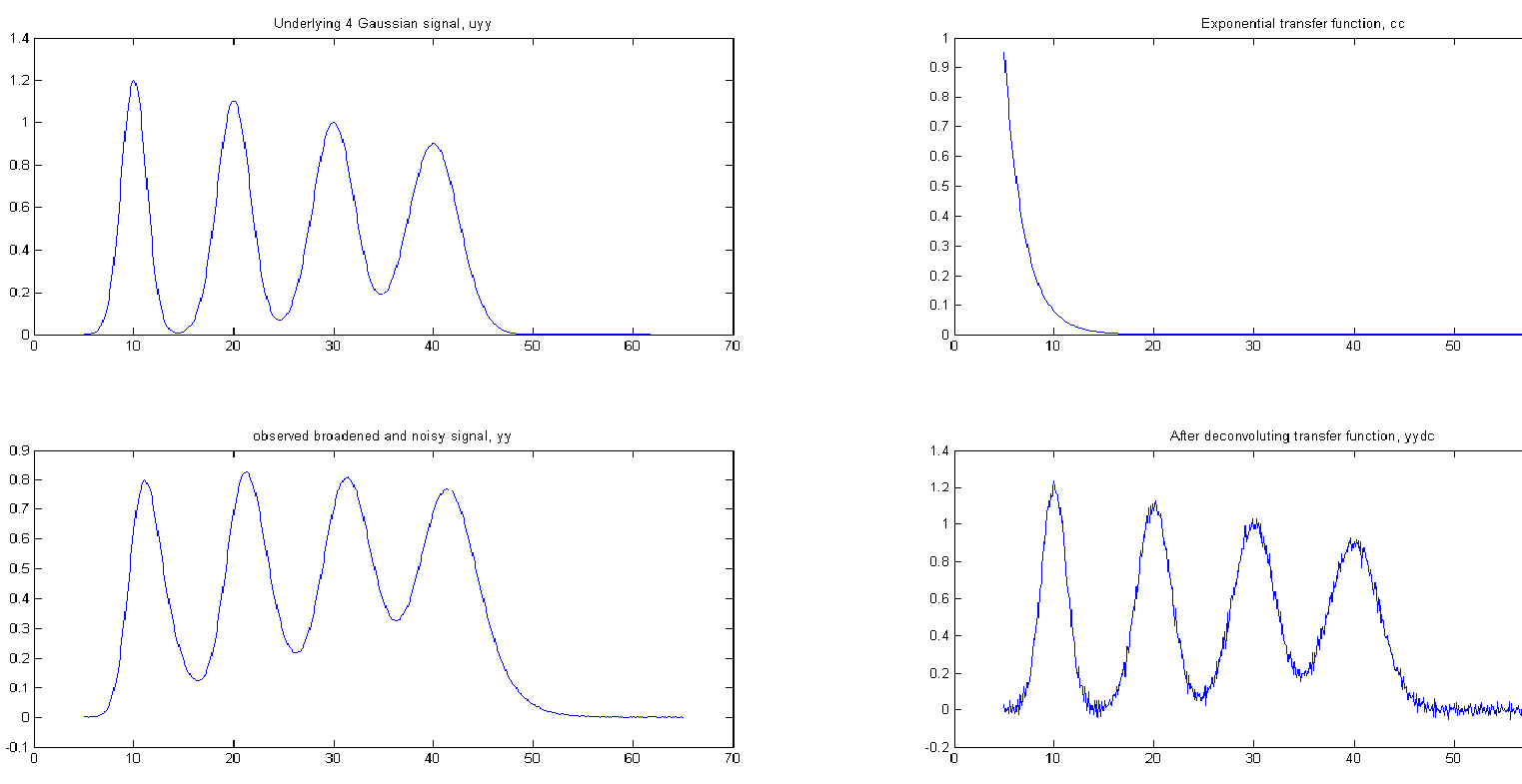
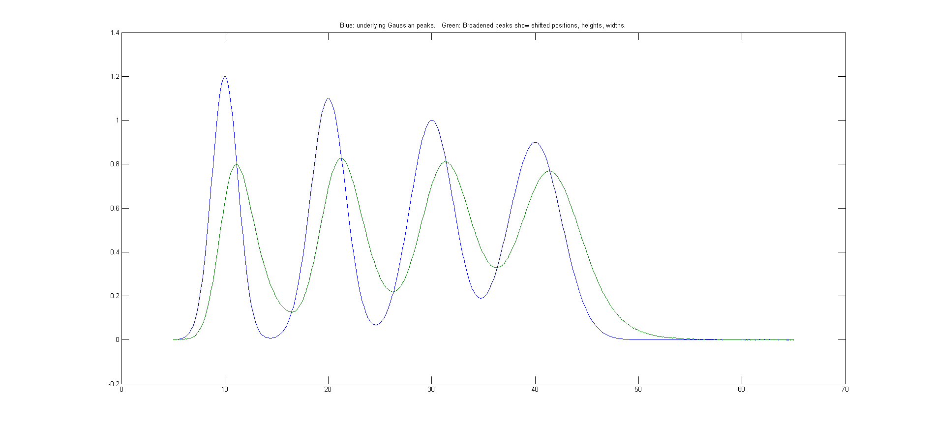
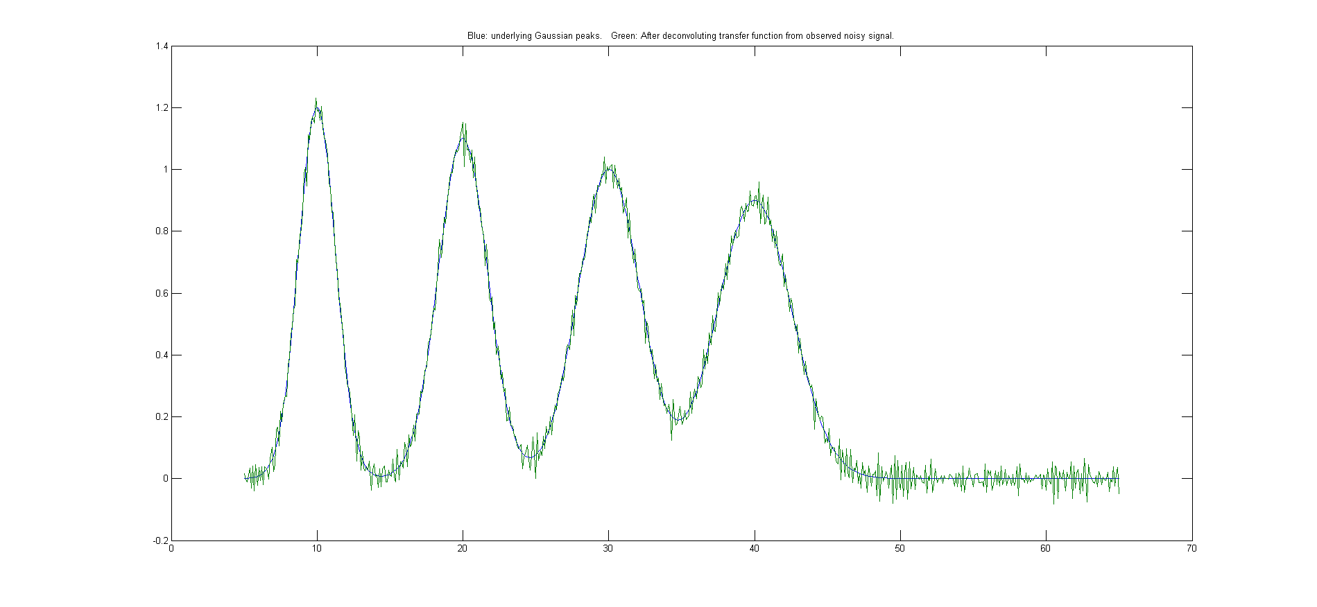
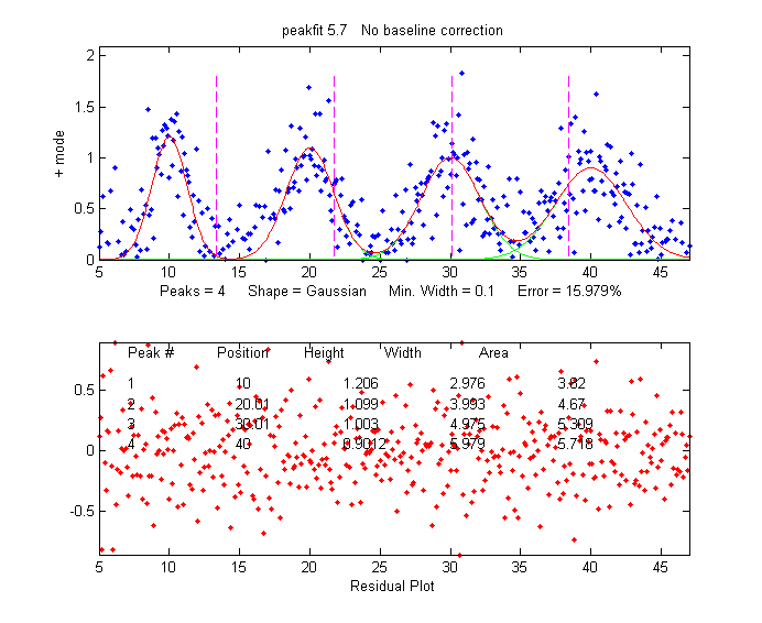
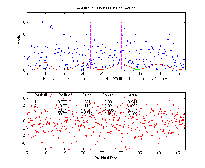
In the script shown below and the resulting graphic shown on the right (Download this script), the underlying signal (uyy) is a set of four Gaussians with peak heights of 1.2, 1.1, 1, 0.9 located at x=10, 20, 30, 40 and peak widths of 3, 4, 5, 6, but in the observed signal (yy) these peaks are broadened exponentially by the exponential function cc, resulting in shifted, shorter, and wider peaks, and then a little constant white noise is added after the broadening. The deconvolution of cc from yy successfully removes the broadening (yydc), but at the expense of a substantial noise increase. However, the extra noise in the deconvoluted signal is high-frequency weighted ("blue") and so is easily reduced by smoothing and has less effect on least-square fits than does white noise. (For a greater challenge, try adding more noise in line 6 or use a bad estimate of time constant in line 10). To plot the recovered signal overlaid with underlying signal: plot(xx,uyy,xx,yydc). To plot the observed signal overlaid with the underlying signal: plot(xx,uyy,xx,yy). Excellent values for the original underlying peak positions, heights, and widths can be obtained by curve-fitting the recovered signal to four Gaussians: [FitResults,FitError]= peakfit([xx;yydc],26,42,4,1,0,10). With ten times the previous noise level (Noise=.01), the values of peak parameters determined by curve fitting are still quite good, and even with 100x more noise (Noise=.1) the peak parameters are more accurate than you might expect for that amount of noise (because that noise is blue). Visually, the noise is so great that the situation looks hopeless, but the curve-fitting actually works pretty well.
xx=5:.1:65;
% Underlying Gaussian peaks with unknown heights,
positions, and widths.
uyy=modelpeaks2(xx,[1
1 1 1],[1.2 1.1 1 .9],[10 20 30 40],[3 4 5 6],...
[0 0 0 0]);
% Observed signal yy, with noise added AFTER the broadening
convolution
Noise=.001; % <---Try more noise to see how this method
handles it.
yy=modelpeaks2(xx,[5 5 5 5],[1.2 1.1 1 .9],[10 20 30
40],[3 4 5 6],...
[-40 -40 -40 -40])+Noise.*randn(size(xx));
% Compute transfer function, cc,
cc=exp(-(1:length(yy))./40); % <---Change exponential
time constant here
% Attempt to recover original signal uyy by deconvoluting
cc from yy
% It's necessary to zero-pad the observed signal
yy as shown here.
yydc=deconv([yy zeros(1,length(yy)-1)],cc).*sum(cc);
% Plot and label everything
subplot(2,2,1);plot(xx,uyy);title('Underlying signal,
uyy');
subplot(2,2,2);plot(xx,cc);title('Exponential transfer
function, cc')
subplot(2,2,3);plot(xx,yy);title('observed broadened,
noisy signal, yy');
subplot(2,2,4);plot(xx,yydc);title('Recovered signal,
yydc')
An alternative to
the above deconvolution approach is to curve fit the
observed signal directly with an exponentially broadened Gaussian
(shape number 5): [FitResults,FitError]=peakfit([xx;yy],26,50,4,5,40,10).
Both methods give good values of the peak parameters, but
the deconvolution method is considerably faster, because
curve fitting with a simple Gaussian model is faster than
fitting with a exponentially broadened peak model,
especially if the number of peaks is large. Also, if the
exponential factor is not known, it can be determined by
curve fitting one or two of the peaks in the observed
signal, using ipf.m, adjusting the exponential factor
interactively to get the best fit. Note that you have to give
peakfit a reasonably good value for the time constant
('extra'), the input argument
right after the peakshape number. If the value is too
far off, the fit may fail completely, returning all zeros. A
little trial and error suffice. Alternatively, you could try
to use peakfit.m
version 7 with the independently
variable time constant exponentially-broadened
Gaussian
shape number 31 or 39, to measure the time constant as an
iterated variable (to understand the difference, see example 39). If the time
constant is expected to be the same for all peaks, better results
will be obtained by using shape number 31 or 39 initially to
measure the time constant of an isolated peak (preferably
one with a good S/N ratio), then apply that fixed time
constant in peak shape 5 to all the other groups of
overlapping peaks.
This page is part of "A Pragmatic Introduction to Signal
Processing", created and maintained by Tom O'Haver, Professor
Emeritus, Department of Chemistry and Biochemistry, The University
of Maryland at College Park. Comments, suggestions and questions
should be directed to Prof. O'Haver at toh@umd.edu. Updated July, 2022.
![FitResults,FitError]= peakfit([xx;yydc],26,42,4,1,0,10)](peakfitxxyydc.png)
![[FitResults,FitError]=peakfit([xx;yy],26,50,4,5,40,10)](yyExpGfit.png)