Fourier convolution is used here to determine how the optical spectrum in Window 1 (top left) will appear when scanned with a spectrometer whose slit function (spectral resolution) is described by the Gaussian function in Window 2 (top right). The Gaussian function has already been rotated so that its maximum falls at x=0, which is necessary to prevent the result from being shifted on the x-axis. The resulting convoluted optical spectrum (bottom center) shows that the two lines near x=110 and 120 will not be resolved but the line at x=40 will be partly resolved. Fourier convolution is used in this way to correct the analytical curve non-linearity caused by spectrometer resolution, in the "Tfit" method for hyperlinear absorption spectroscopy.
Simple whole-number convolution vectors:
Smoothing
3 point boxcar (sliding average) smooth
[1 1 1]
4 point boxcar (sliding average)
smooth
[1 1 1 1]
3 point triangular smooth
[1 2 1]
5 point triangular smooth
[1 2 3 2 1]
5 point Gaussian
smooth
[1 4 6 4 1]
7 point Gaussian smooth
[1 4 8 10 8 4 1]
9 point Gaussian
smooth
[1 4 9 14 17 14 9 4 1]
Differentiation:
[-1 1]
First derivative
[1 -2 1]
Second derivative
[1 -3 3 -1]
Third derivative
[1 -4 6 -4 1] Fourth derivative
Results of successive convolution by two
vectors Conv1 and Conv2:
(⁕ stands for convolution)
Conv1
Conv2
Result
Description
[1 1 1] ⁕ [1 1 1] =
[1 2 3 2 1]
Triangular smooth
[1 2 1] ⁕ [1 2 1] =
[1 4 6 4 1] P-spline
smooth
[-1 1] ⁕ [-1
1] = [1 -2
1]
2nd derivative
[-1 1] ⁕ [1 -2 1] =
[1 -3 3 -1] 3rd
derivative
[1 -2 1] ⁕ [1 -2 1] = [1 -4 6 -4
1] 4th
derivative
[-1 1] ⁕ [1 1
1] = [1 0 0
-1) 1st
derivative gap-segment
[-1 1] ⁕ [1 2
1] = [1 1 -1
-1) Smoothed 1st
derivative
[1 1 -1 -1] ⁕ [1 2 1] = [1 3 2 -2 -3
-1] Same with more smoothing
[1 -2 1] ⁕ [1 2 1] = [1 0
-2 0 1] 2nd derivative
gap-segment
[1 1 1 1] ⁕ [1 1 1 1] = [1 2 3 4 3 2
1] 2 passes of 4-point sliding
average
rectangle conv rectangle = triangle or trapezoid (depends
on relative widths)
Gaussian conv Gaussian = Gaussian of greater width
Gaussian conv Lorentzian = Something in between Gaussian
and Lorentzian
Spreadsheets can be used to perform "shift-and-multiply" convolution for digitally sampled data sets (for example, MultipleConvolution.xlsx, MultipleConvolutionFirstDerivativeDemo.xls (screen shot), and MultipleConvolution4thDerivativeDemo.xls (screen shot) for Excel and MultipleConvolutionOO.ods for Calc). For very large data sets the performance can be much slower that Fourier convolution (which is much easier done in Matlab/Octave or in Python than in spreadsheets). Spreadsheets, however, do have the instructional advantage of showing the "shift-and-multiply" operation more clearly and explicitly.
 A good example of this
occurs in the technique of twin-column recycling separation process
(TCRSP), a novel chromatography technique in which the injected
sample is recycled back to the two columns for obtaining better and
better resolution, allowing chromatographers to solve challenging
separation problems caused by the partition coefficients for the
components being too similar and/or too low column efficiencies
[reference 90]. In TCRSP, after the sample is separated by the first
column, it flows into the second identical column, and after that
separation, switching valves connect it back into the first column.
That cycle repeats as many times as required. Each pass through a
column increases the separation between the components slightly, so
that with a sufficiently large number of cycles, very similar
substances can be separated. As described in a later section, chromatographic separations
often involve broadening of the peaks by asymmetrical mechanisms,
usually modeled as an exponentially modified Gaussian (EMG). Any
broadening that occurs in the first pass will occur repeatedly in
the subsequent passes. The net result will be a final peak shape
that cannot be described by a single convolution. The success of the
TCRSP technique depends on the fact that the separation between the
components increases faster than the width increase caused by the
successive convolutions of broadening mechanisms.
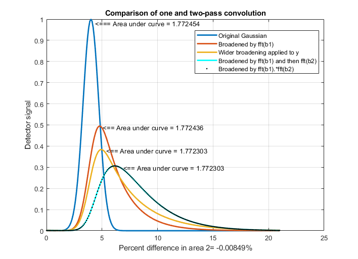
  This is demonstrated by the simple example of
two sequential exponential convolutions applied to a Gaussian, as
shown in the figure on the left, generated by a Matlab/Octave script. The blue
curve is the original Gaussian. The red curve is the result of a
single convolution by an exponential function whose time constant tau
is 2. The cyan curve is the result of two successive convolutions
with that same tau. The orange curve is an attempt to
duplicate that with a single wider convolution of tau equal
to 3. That attempt fails; the result is a poor match to the cyan
curve. In fact, experiments show that no single wider
exponential convolution can match the result of two (or more)
successive convolutions; the shape is fundamentally different.
Multiple exponential convolutions result in a less asymmetrical
peak, more shifted to larger x values. On the other hand, a single
convolution by a function that is the product of the Fourier
transforms of the two separate functions does work (black dots).
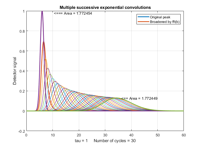
With greater numbers of successive convolutions, the peaks become
progressively more symmetrical and more Gaussian as the number
of cycles increases, as demonstrated for 30 cycles by the figure on
the right, which was created by this Matlab/Octave script (where you
can choose the number of convolutions in line 20).
