Command-line Fourier filter function for time-series signal vector y; 'samplingtime' is the total duration of sampled signal in sec, millisec, or microsec; 'centerfrequency' and 'frequencywidth' are the center frequency and width of the filter in Hz, KHz, or MHz, respectively. If 'shape' = 1, the filter is Gaussian; as 'shape' increases, the filter shape becomes more and more rectangular (faster cut-off rate). Set 'mode' = 0 for band-pass filter, 'mode' = 1 for band-reject (notch) filter. Click here to view or download just this function.
Example: plot(FouFilter(tan(1:1000),15,2,2,0))
iFilter is a
keyboard-operated interactive Fourier filter function for
time-series signal (x,y), with keyboard controls that allow you to
adjust the filter parameters continuously while observing the
effect on your signal dynamically. Optional input arguments set
the initial values of center frequency, filter width, shape,
plotmode (1=linear; 2=semilog frequency; 3=semilog amplitude;
4=log-log) and filter mode ('band-pass', 'low-pass', 'high-pass',
'band-reject (notch), 'comb pass', and 'comb notch'). In the comb
modes, the filter has multiple bands located at frequencies 1, 2,
3, 4... times the center frequency, each with the same
(controllable) width and shape.
The filtered signal can be returned as the function value, saved
as a ".mat" file on the disk, or plays through the computer's
sound system. Press K to list keyboard commands.
This is a self-contained Matlab function that does not require any
toolboxes or add-on functions. Click here
to view or download and place it in the Matlab path.
At the Matlab command prompt, type: ifilter(x,y) or ifilter(y) or ifilter(xymatrix) or
ry=ifilter(x,y,center,width,shape,plotmode,filtermode)
Version 4.3, June 2016
Example 1:
Periodic waveform with 2 frequency components at 60 and 440
Hz.
x=[0:.001:2*pi];
y=sin(60.*x.*2.*pi)+2.*sin(440.*x.*2.*pi);
ifilter(x,y);
Example 2: uses optional input arguments to set initial
values:
x=0:(1/8000):.3;
y=(1+12/100.*sin(2*47*pi.*x)).*sin(880*pi.*x)+(1+12/100.*sin(2*20*pi.*x)).*sin(2000*pi.*x);
ry=ifilter(x,y,440,31,18,3,'Band-pass');
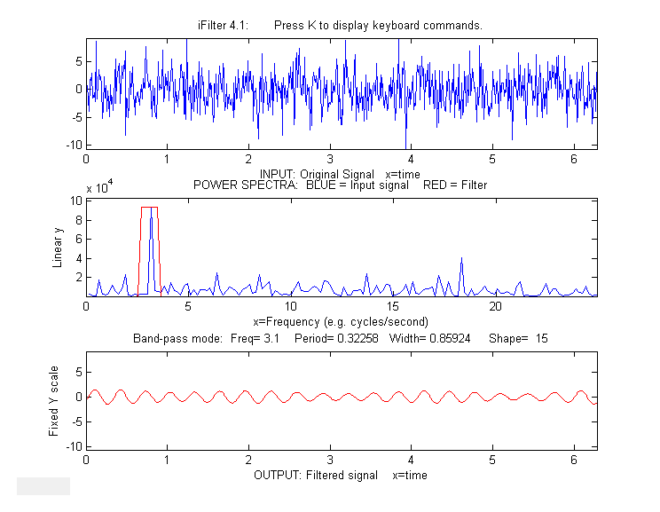
Example 3: Picking one frequency out of a noisy sine wave.
x=[0:.01:2*pi]';
y=sin(20*x)+3.*randn(size(x));
ifilter(x,y,3.1,0.85924,15,1,'Band-pass');
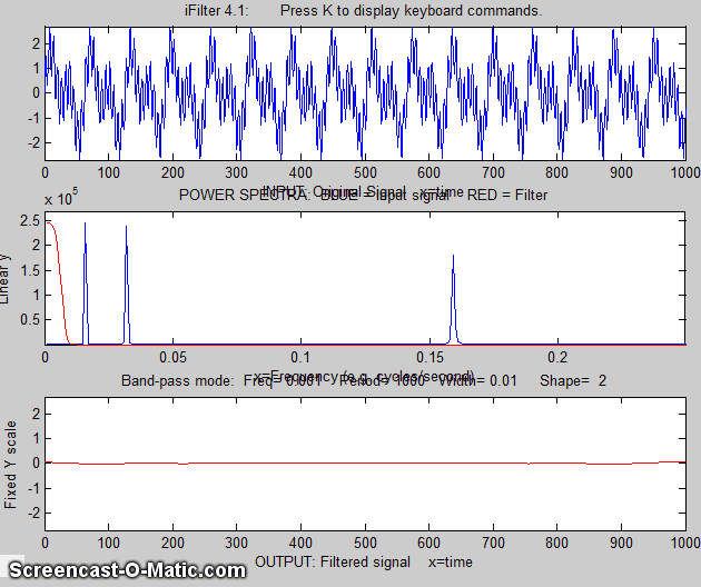
Example 4: Square wave with band-pass vs Comb pass filter
t = 0:.0001:.0625;
y=square(2*pi*64*t);
ifilter(t,y,64,32,12,1,'Band-pass');
ifilter(t,y,48,32,2,1,'Comb
pass');
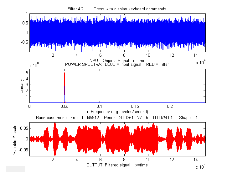
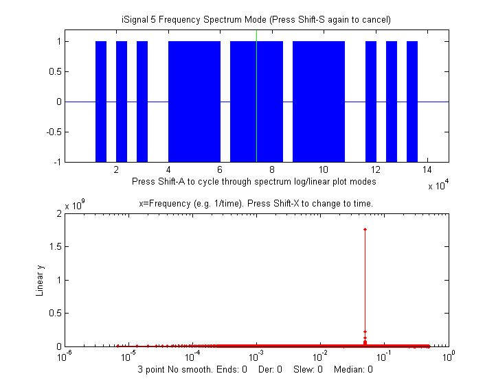
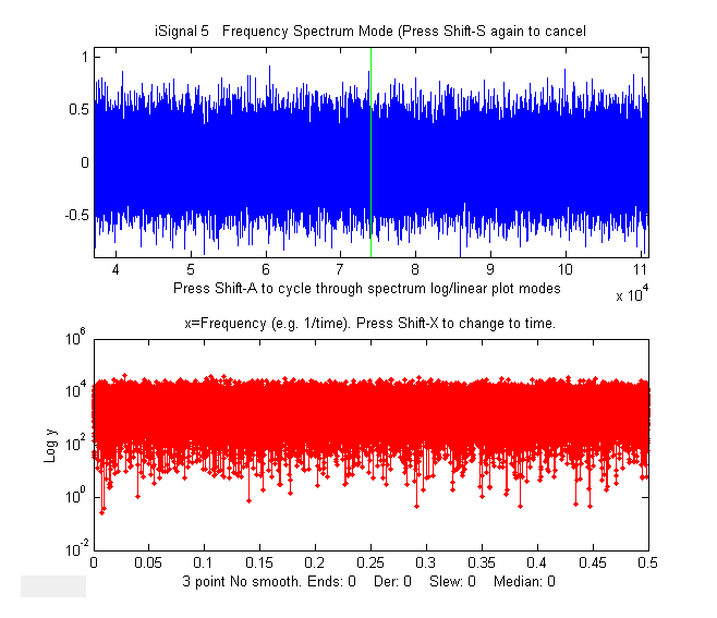
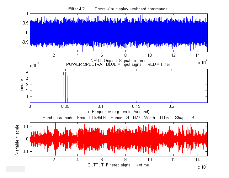
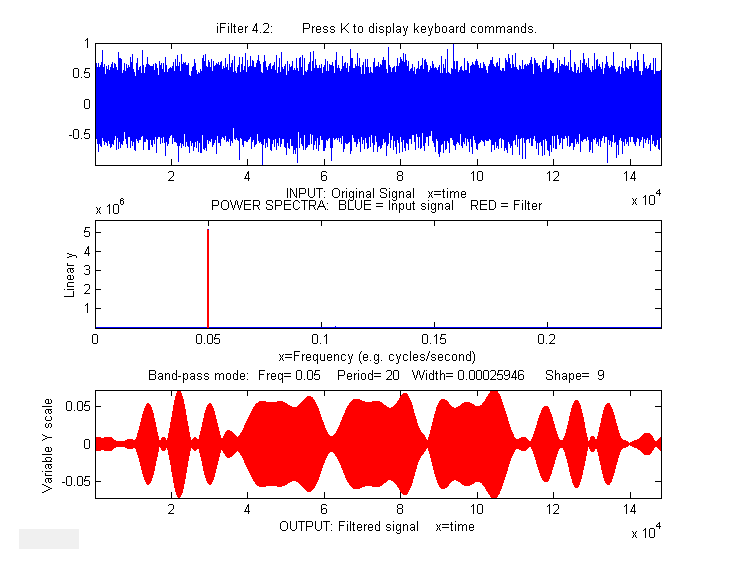
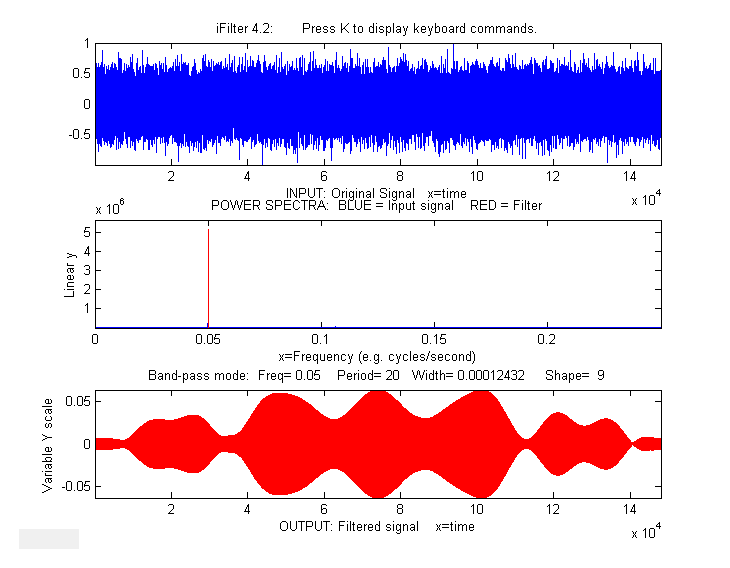
Example 5: MorseCode.m uses iFilter to demonstrate
the abilities and limitations of Fourier filtering. It creates a
pulsed fixed frequency (0.05) sine wave
that spells out "SOS" in Morse code
(dit-dit-dit/dah-dah-dah/dit-dit-dit), adds random white noise so
that the SNR is very poor
(about 0.1 in this example). The white noise has a frequency
spectrum that is spread out over
the entire range of frequencies; the signal itself is
concentrated mostly at a fixed frequency (0.05) but the
modulation of the sine wave by the Morse Code pulses spreads
out its spectrum over a narrow
frequency range of about 0.0004. This suggests that a
Fourier bandpass filter tuned to the signal frequency might be
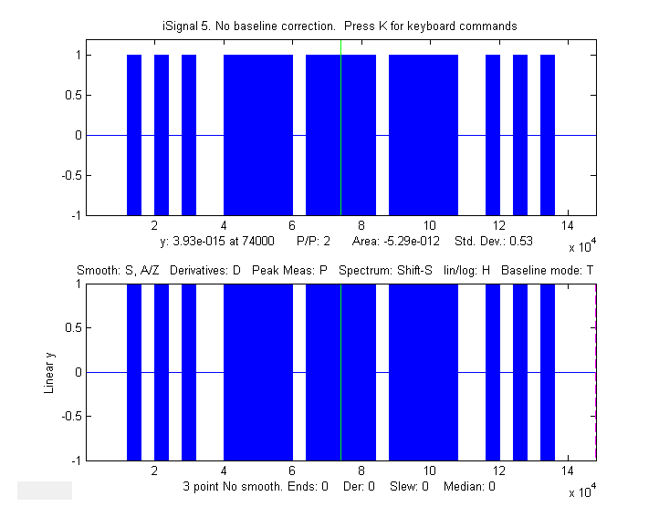
able to isolate the signal from the noise. As the bandwidth is reduced, the
signal-to-noise ratio improves and the signal begins to emerges from the
noise until it
becomes clear, but if the bandwidth is too narrow,
the step response time is too slow to give distinct "dits"
and "dahs". The step response time is inversely proportional to
the bandwidth. (Use the ? and " keys to adjust the bandwidth.
Press 'P' or the Spacebar to hear the sound). You can
actually hear that sine wave component better than you
can see it in the waveform plot (upper panel), because the
ear works like a spectrum analyzer, with separate nerve
endings assigned to to specific frequencies, whereas the eye
analyzes the graph spatially, looking at the overall amplitude and
not at individual frequencies. Watch
an mp4 video of this script in operation, with sound. Also on YouTube.
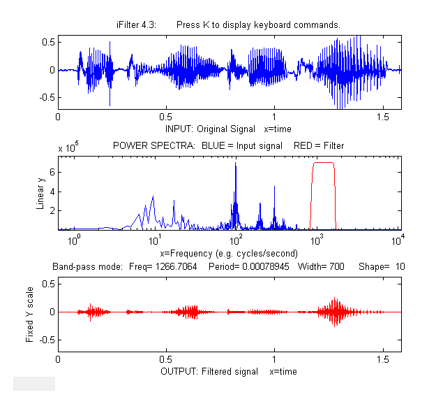
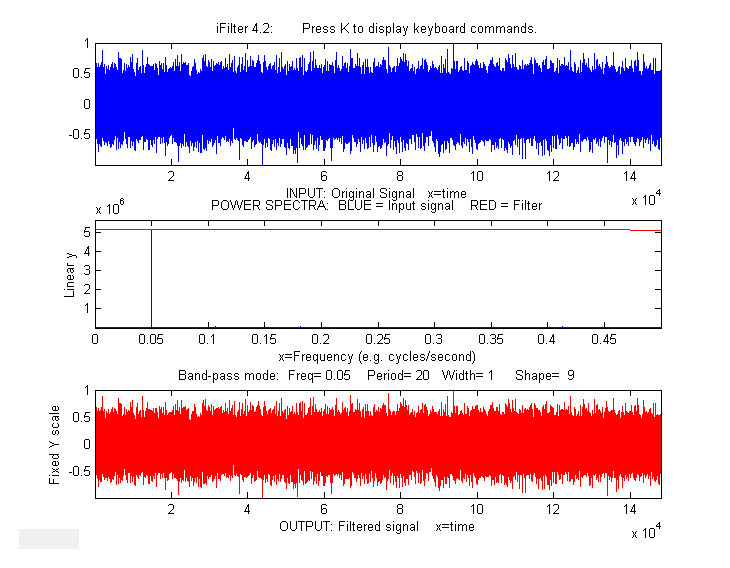
Example
6: This example shows a 1.58 sec duration
audio recording of the spoken phrase "Testing, one, two, three",
previously recorded at 44000 Hz and saved in WAV format (download link) and in ".mat"
format (download link), loaded into iFilter, which is initially set to bandpass
mode and tuned to a narrow segment that is well above the
frequency range of most of the signal. It seems as if though this
passband would miss most of the frequency components in the
signal, yet even in this case the speech is intelligible,
demonstrating the remarkable ability of the ear-brain system to
make do with a highly compromised signal. Press P or space
to hear the filter's output. Different filter settings will
change the timbre
of the sound.
>> v=wavread('TestingOneTwoThree.wav');
>> time=0:1/44001:1.5825;
>> waveform=v(:,2);
>> ifilter(time,waveform,1267,700,10,2,'Band-pass');
iFilter 4.3 KEYBOARD CONTROLS when figure window is
topmost
Adjust filter frequency.......Coarse (10% change): < and >
Fine (1% change): left and right cursor
arrows
Adjust filter width...........Coarse (10% change): / and "
Fine (1% change): up and
down cursor arrows
Filter shape..................A,Z (A
more rectangular, Z
more Gaussian)
Filter mode...................B=bandpass; N
or R=notch (band
reject);H=High-pass;
L=Low-pass; C=Comb pass; V=Comb notch.
Select plot mode..............1=linear; 2=semilog
frequency
3=semilog amplitude; 4=log-log
Print keyboard commands.......K Pints this list
Print filter parameters.......Q or W Prints ifilter with input
arguments: center, width, shape,
plotmode, filtermode
Print current settings........T Prints list of current settings
Switch SPECTRUM X-axis scale..X switch between frequency and period
on the horizontal axis
Switch OUTPUT Y-axis scale....Y switch output plot between fixed or
variable
vertical axis.
Play output as sound..........P or Enter
Save output as .mat file......S
This page is part of "A Pragmatic Introduction to Signal Processing", created and maintained by Prof. Tom O'Haver , Department of Chemistry and Biochemistry, The University of Maryland at College Park. Comments, suggestions and questions should be directed to Prof. O'Haver at toh@umd.edu.
Last updated: December, 2021. Number of unique visits to this site since May 17, 2008: