


Z. Dealing with variable data arrays in spreadsheets
When applying spreadsheet templates of the type
described in this book to your own data, it's often necessary to
modify the templates to accommodate different numbers of data
points or of components. This can be tedious to do, especially
because you need to remember the syntax of each of the spreadsheet
functions that you want to modify. This section describes ways to
construct spreadsheets that automatically adapt to different data sets, without
your taking the time and effort to modify the spreadsheet formulas
for each case. This involves employing some less commonly used
built-in functions in Excel or OpenOffice Calc, such as MATCH,
INDIRECT, COUNT, IF, and AND.
The MATCH function. In
signal processing using spreadsheets, it's common to have x-y
arrays of data of variable length, such as spectra
(x=wavelength, y=absorbance or intensity) or chromatograms
(x=time, y=detector response). For 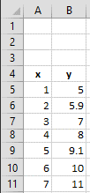 example,
consider this small array of x and y values pictured in the
spreadsheet fragment on the left. Spreadsheet formulas normally
refer to cells by their row and column address, but for an x-y
data set like this, it's more natural to refer to a data point
by its independent variable x, rather than its row and column
address. For example, suppose you want to select the data point
where x=2, irrespective of what cells they inhabit. You
can do that with the MATCH function. For example, if you set
cell B2 to the desired x value (2), then the cell formula
MATCH(B2,A5:A11) + ROW(A5) will return the row number of that
point, which is 6 in this case. Later, if you were to move or
expand this table, by dragging it or by inserting or deleting
rows or columns, the spreadsheet will automatically adjust the
MATCH function to compensate, returning the new row number of
the requested point.
example,
consider this small array of x and y values pictured in the
spreadsheet fragment on the left. Spreadsheet formulas normally
refer to cells by their row and column address, but for an x-y
data set like this, it's more natural to refer to a data point
by its independent variable x, rather than its row and column
address. For example, suppose you want to select the data point
where x=2, irrespective of what cells they inhabit. You
can do that with the MATCH function. For example, if you set
cell B2 to the desired x value (2), then the cell formula
MATCH(B2,A5:A11) + ROW(A5) will return the row number of that
point, which is 6 in this case. Later, if you were to move or
expand this table, by dragging it or by inserting or deleting
rows or columns, the spreadsheet will automatically adjust the
MATCH function to compensate, returning the new row number of
the requested point.
The INDIRECT function.
The usual way to reference the value in a cell is to specify its
row and column address. For example, take the small array of x and
y values pictured above. To refer to the contents of column B, row
6, you could write "=B6", which in this case will evaluate to 5.9.
This is referred to as "direct" addressing. In contrast, to use
"indirect" addressing you can write "=INDIRECT("B"&A1)",
then put the number "6" in cell A1. The "&" character is
simply "glue" that joins "B" to the contents of A1, so in that
case "B"&A1 evaluates to "B6" and the result is the same as
before: the contents of cell B6, which is 5.9. However, if you change
cell A1 to 9, then "B"&A1 would evaluate to "B9", and the
result would be the contents of cell B9, which is 9.1. In other
words, the indirect function allows the addresses of cells to be calculated within the
spreadsheet rather than being typed in as a fixed number.
This makes it possible for spreadsheets to adjust their own
addresses based on a calculated result, for example to adapt their
calculations to fit the number of data points in that particular
data set.
These examples were done in what is called the "A1" reference
style, where the columns are referred to by letters; it's also
possible to use the "R1C1" reference style, where both the and the
rows columns are referred to by numbers. For example
=INDIRECT("R"&A2&"C"&A1,FALSE)",
with the row number in A2 and the columns number in A1. (The
"FALSE" just means that the "R1C1" reference style is used). The "R1C1" reference style allows both the row
and column address to be expressed as numbers that can be
calculated within the spreadsheet.
You can use the same
technique to compute ranges
of cell addresses. For example, you could compute the sum of the y
values in column B, rows 5 to 11, by writing SUM(B5 : B11) by
direct addressing. But suppose you wanted to compute the sum of
all the numbers in column B between a variable first row
and variable last row. If you put the first row number in
A1 and the last row number in row A2, the address of the first cell would be
"B"&A1 and the address of the last cell would be
"B"&A2. So you would form the range of cell addresses by using
"&" to glue together those two addresses, with a colon
in-between ("B"&A1&" : B"&A2). The sum would be
SUM(INDIRECT("B"&A1&" : B"&A2)), which is 56. Yes,
it's longer, but the advantage over direct addressing is that you
can adjust the range by changing just two cells rather that
retyping the formula. It's the same for other functions that need
a range of cells, such as AVERAGE, MAX, MIN, STDEV, etc. For
examples of its use in signal processing, see VariableSmooth.xlsx
(screen
image).
For functions that
require two ranges,
separated by a comma, you can use the same technique. For example.
suppose you want to compute the slope
of the linear regression line between the x values in column A and
the y values in column B in the spreadsheet except in the previous
figure, using the built-in SLOPE function. SLOPE requires two
ranges, first the dependent (y) values and them the independent x
values. By direct
addressing, the slope is SLOPE(B5 : B11,A5 : A11) .
By indirect addressing,
you need two separate "indirect" functions, one for each range,
separated by a comma. Here's what it looks like all together:
SLOPE(INDIRECT("B"&A1&" : B"&A2),
INDIRECT("A"&A1&" : A"&A2)), where the x
values are in column A, the y values in column B, and the first
and last row numbers are in cells A1 and A2 respectively. It works
exactly the same for the two related functions that calculate the
INTERCEPT and RSQ (the R2 value) of the regression line. I admit
that the formula is confusing to read at first, but it works. Just
break it down into its parts.
A working example. An
example of the use of the MATCH and INDIRECT functions working
together is demonstrated in the spreadsheet "SpecialFunctions.xlsx"
(Graphic),
which
has a larger table of x-y data stored in columns A and B, starting
in row 7. The idea here is that you can select a limited range of
x values to work with by typing in the lowest x and the highest x value in cells B2 and
B3, the two cells with a 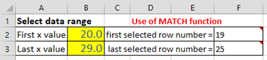 yellow background,
shown on the left. The spreadsheet uses the MATCH functions in
cells F2 and F3 to compute the corresponding row numbers, which
are then used in the INDIRECT functions in the "Properties of
selected data range" section to compute the maximum, average,
and average of x and of y, and also the slope, intercept,
and R2 values of the y vs x linear regression line over that
selected x interval. The regression line, fitting only the data from x=20
to 29, is shown in red in the graph on the right, superimposed
on the complete data set (blue dots). By simply changing the
yellow background,
shown on the left. The spreadsheet uses the MATCH functions in
cells F2 and F3 to compute the corresponding row numbers, which
are then used in the INDIRECT functions in the "Properties of
selected data range" section to compute the maximum, average,
and average of x and of y, and also the slope, intercept,
and R2 values of the y vs x linear regression line over that
selected x interval. The regression line, fitting only the data from x=20
to 29, is shown in red in the graph on the right, superimposed
on the complete data set (blue dots). By simply changing the 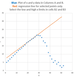 x-axis limits in cells B2 and B3, the spreadsheet and the graph
re-calculates, without your having to edit any of the cell
formulas. Try it yourself. (Hint: Cells with red mark in
upper right corner contain helpful pop-up notes: you can float the mouse pointer over any
such cell to reveal its cell formula and/or an
explanation).
x-axis limits in cells B2 and B3, the spreadsheet and the graph
re-calculates, without your having to edit any of the cell
formulas. Try it yourself. (Hint: Cells with red mark in
upper right corner contain helpful pop-up notes: you can float the mouse pointer over any
such cell to reveal its cell formula and/or an
explanation).
Columns J and K of this sheet also show how to use the "IF" and
"AND" functions to copy data from columns A and B into columns J
and K only those data points that fall between the two specific x
limits.
If desired, you can add more data to the end of columns A and B,
limited only be the range of the match functions in cells F2 and
F3 (which are initially set to 1000, but that could be as large as
you need). The total number of numerical values in the data set is
computed in cell I15, using the "COUNT" function (which, as the
name suggests, counts the number of cells in a range that contains
numbers and does not count empty cells or cells with letters).
Measuring peak location.
A common signal processing operation is finding the x-axis value
where the y-axis value is maximum. This can be broken down into
four steps:
(1) Define the range of values, either directly or
using the indirect function, e.g. INDIRECT("B"&F2&":B"&F3)
(2) Determine the maximum y
value in that range with the
MAX function,
e.g.: MAX(INDIRECT("B"&F2&":B"&F3))
(3) Determine the row number in which that number
appears
with the MATCH function, e.g.: MATCH(H20,B7:B1000,0)+ROW(A6)
(4) Determine the value of x in that row with the
INDIRECT function,
e.g.: INDIRECT("A"&H21)
Each step references the results of the one before
it. These steps are illustrated in the same "SpecialFunctions.xlsx"
spreadsheet in column H, rows 20-23. The result is that the
maximum y (21.5) occurs at x=28. These steps can even be combined
into one long formula (cell H23), although this is harder to read,
and harder to document, than the formulas for the separate steps.
The peak finder spreadsheet uses this
technique.
The LINEST function.
Indirect addressing is particularly useful when using array functions such as
LINEST or the matrix algebra functions. The demonstration
spreadsheet "IndirectLINEST.xlsx"
(graphic
link) shows how this works for the multiwavelength
spectroscopy analysis of a mixture of three overlapping components
by the CLS method. The measured mixture spectrum is in column C,
rows 29-99 and the spectra of the three pure components are in
columns D, E, and F. Cell C12 "=COUNT(C29:C1032)"
counts the number of rows of data (i.e. number of wavelengths) in column C
starting at row 29, and cell G3 counts the number of components (in this case
3). These are used to determine the first and last row and column
for the indirect addresses in LINEST in cell C17. The measured
peaks heights calculated by LINEST for the three peaks are given
in row 17, columns C, D, can E, and the predicted standard
deviations are in the row below. In this spreadsheet the data are
actually simulated
(over in columns O - U), so the true peaks heights are known and
therefore the absolute
accuracy can be calculated (row 26, C, D, and E) and
compared to the predicted standard deviations. Press the F9 key to recalculate
with an independent noise sample, which is equivalent to taking
another measurement of the same sample. Because of the use of
INDIRECT addressing, you can add or subtract data points at the
end of columns C - E and the calculations work with no other
changes. Examples of its use in signal processing are on CurveFittingB.html#spreadsheets.
This page is part of "A Pragmatic Introduction to Signal
Processing", created and maintained by Prof. Tom O'Haver ,
Department of Chemistry and Biochemistry, The University of Maryland
at College Park. Comments, suggestions and questions should be
directed to Prof. O'Haver at toh@umd.edu. Updated July, 2022.