


Appendix Y: Real-time signal
processing
All of the signal processing techniques
covered so far make the assumption that you have acquired and
stored the data in computer memory before beginning processing. In
some cases, however, it is necessary to do the signal processing
in "real time", that is, point-by-point as the data are acquired
from the sensor or instrument. That requires some modification of
the software, but the main ideas still apply. In this section we
will look at ways to perform real-time data plotting, smoothing,
differentiation, peak detection, harmonic analysis (frequency
spectra), and Fourier filtering. Because the details of the data
acquisition itself varies with each individual experimenter and
instrumental setup, these demonstration scripts will simulate real-time
data so that you can run them immediately on
your computer without additional hardware. I'll do this in either
of two ways:
(a) by using mouse-clicks to generate
each data point, using Matlab's "ginput" function, or
(b) by pre-calculating simulated data and then
accessing it point-by-point in a loop.
The first method is illustrated by the
simple script realtime.m.
When you run this script, it displays a graphical coordinate
system; position your mouse pointer along the y (vertical)
axis and click to enter data points as you move the mouse pointer
up and down. The "ginput" function waits for each click of the
mouse button, then the program records the y coordinate
position and counts the number of clicks. Data points are assigned
to the vector y (line 17), plotted on the graph as black
points (line 18), and print out in the command window (line 19). The script realtimeplotautoscale.m is an
expanded version that changes the graph scale as the data come in.
If the number of data points exceeds 20 ('maxdisplay'), the x
axis maximum is re-scaled to twice that (line 32). If the
data amplitude equals or exceeds ('maxy'), the y axis is
re-scaled to 1.1 times the data amplitude (line 36).
 The script realtimeplotautoscale2.m
uses the second method to simulate real-time
data, using pre-calculated data (loaded from
disk in line 13) that is accessed point-by-point in lines 25 and
26 (animation shown on the right).
The script realtimeplotautoscale2.m
uses the second method to simulate real-time
data, using pre-calculated data (loaded from
disk in line 13) that is accessed point-by-point in lines 25 and
26 (animation shown on the right).
The script realtimeplotdatedtime.m demonstrates
one way to use Matlab's 'clock' function to record the data and
time of each data point that is acquired by clicking. You could
also have the computer control the time of data acquisition by
reading the clock in a loop until the desired time and date
arrives, then take a data point. Of course, a Windows machine is
not ideal for high-speed, precisely-timed data acquisition,
because there are typically so many interrupts and other processes
going on in the background, but it's adequate for low-speed
applications. For higher speeds, specialized
hardware and software is
available.
Smoothing. The script RealTimeSmoothTest.m
demonstrates real-time smoothing,
plotting the raw unsmoothed data as a black line and the smoothed
data in red. In this case the script pre-calculates
simulated data in line 28 and then accesses the data
point-by-point in the processing 'for' loop (lines 30-51).
The total number of data points is controlled by 'maxx' in line 17
(initially set to 1000) and the smooth width (in points) is
controlled by 'SmoothWidth' in line 20. (To do this with real time
data from your sensor, comment out line 29 and replace line 32
with the code that acquires one data point from your sensor).
 As you can see in the
screen animation on the left, the smoothed
data (in red) is delayed compared to the raw data, because a
smoothed data point can not be computed until a number of data
points equal to the smooth width has been acquired - 21 points, or
about 0.5 seconds in this example. (However, knowing the smooth
width, you can correct the recorded y-axis positions of signal
features, such as maxima, minima, peaks, or inflection points).
This particular example implements a sliding
average smooth, but other smooth shapes can be implemented
simply by uncommenting line 24 (rectangular smooth), 25 (triangular smooth),
or 26 (Gaussian smooth), which requires
that the functions 'triangle'
and 'gaussian' be
in the Matlab/Octave path.
As you can see in the
screen animation on the left, the smoothed
data (in red) is delayed compared to the raw data, because a
smoothed data point can not be computed until a number of data
points equal to the smooth width has been acquired - 21 points, or
about 0.5 seconds in this example. (However, knowing the smooth
width, you can correct the recorded y-axis positions of signal
features, such as maxima, minima, peaks, or inflection points).
This particular example implements a sliding
average smooth, but other smooth shapes can be implemented
simply by uncommenting line 24 (rectangular smooth), 25 (triangular smooth),
or 26 (Gaussian smooth), which requires
that the functions 'triangle'
and 'gaussian' be
in the Matlab/Octave path.
A practical application of a sliding average smooth like this is
in a control system where a noisy signal turns on a valve, switch
or alarm signal whenever the signal exceeds a certain value; an
example is shown in the figure on the right,  where the
threshold value is 0.5 and the signal is so noisy that smoothing
is required to prevent the signal from prematurely triggering the
control. Too much smoothing, however, will cause an unacceptable
delay in operation.
where the
threshold value is 0.5 and the signal is so noisy that smoothing
is required to prevent the signal from prematurely triggering the
control. Too much smoothing, however, will cause an unacceptable
delay in operation.
On a standard desktop PC (Intel Core i5 3 Ghz) running
Windows 10 home, the smooth operation adds about 2 microseconds per data point to
the data acquisition time (without plotting, PlottingOn=0) and 20 milliseconds
per point (50 Hz) with point-by-point plotting (PlottingOn=1). With plotting off, the script acquires, smooths, and stores the smoothed data in the
variable "sy" in real time, then plots the data only after data
acquisition is complete, which is much faster than plotting in
real time.
Differentiation . The script RealTimeSmoothFirstDerivative.m
demonstrates real-time smoothed differentiation, using a simple
adjacent-difference algorithm (line 47) and plotting the raw data
as a black line and the first derivative data in red. The
demonstration script RealTimeSmoothSecondDerivative.m computes the smoothed second derivative
by using a central difference algorithm (line 47). Both of
these scripts pre-calculate the simulated data in line 28 and
then accesses the data point-by-point in the processing
loop (lines 31-52). In both cases the
maximum number of points is set in
line 17 and the smooth width is set in line
20. Again,
the derivatives are delayed
compared to the original
signal. Any derivative order
can be calculated this way
using the derivative
coefficients in the
Matlab/Octave derivative
functions listed on Differentiation.html#Matlab.
. The script RealTimeSmoothFirstDerivative.m
demonstrates real-time smoothed differentiation, using a simple
adjacent-difference algorithm (line 47) and plotting the raw data
as a black line and the first derivative data in red. The
demonstration script RealTimeSmoothSecondDerivative.m computes the smoothed second derivative
by using a central difference algorithm (line 47). Both of
these scripts pre-calculate the simulated data in line 28 and
then accesses the data point-by-point in the processing
loop (lines 31-52). In both cases the
maximum number of points is set in
line 17 and the smooth width is set in line
20. Again,
the derivatives are delayed
compared to the original
signal. Any derivative order
can be calculated this way
using the derivative
coefficients in the
Matlab/Octave derivative
functions listed on Differentiation.html#Matlab.
Peak detection. The little script realtimepeak.m
demonstrates simple real-time peak
detection
based on
derivative zero-crossing, using mouse clicks to simulate data. Each
time your mouse clicks form a peak (that is, go up and then down
again), the program will register and label the peak on the
graph and print out its n and y values.
Peak detected at n=13 and y=7.836
Peak detected at n=26 and y=1.707
In this case, a peak
is defined as any data point that has lower amplitude points
adjacent to it on both sides, which is determined by the nested
'for' loops in lines 31-36. Of course, a peak can not be
registered until the point following the peak is recorded,
because there is no way to predict ahead of time whether that
point will be lower or higher than the previous point.
If the data are noisy, it's better to smooth the data stream
before detecting the peaks, which is exactly what RealTimeSmoothedPeakDetection.m
does, which reduces the chance of false peaks due
to random noise but has
the disadvantage of delaying the peak detection further. Even
better, the script RealTimeSmoothedPeakDetectionGauss.m
uses the technique described on PeakFindingandMeasurement.htm#findpeaks;
it locates the positiv e peaks in a noisy data set that rise
above a set amplitude threshold ("AmpThreshold" in line 55),
performs a least-squares curve-fit of a Gaussian
function to the top part of the raw data peak (in line
58), identifies each peak (line 59), computes the position,
height, and width (FWHM) of each peak from that least-squares
fit, and prints out each peak found in the command window. The peak parameters are measured on the raw
data, so they are not distorted by smoothing. If you
look at the animation on the right, you can see that the "peak"
label appears next to each detected peak just a fraction of a
second after the top of the peak, but the actual peak times
listed are not delayed. In this example, the actual peak times
are x=500, 1000, 1100, 1200, 1400. (Also note that the first
visible peak, at x=300, is not detected because it falls below
the amplitude threshold, which is 0.1
in this case).
e peaks in a noisy data set that rise
above a set amplitude threshold ("AmpThreshold" in line 55),
performs a least-squares curve-fit of a Gaussian
function to the top part of the raw data peak (in line
58), identifies each peak (line 59), computes the position,
height, and width (FWHM) of each peak from that least-squares
fit, and prints out each peak found in the command window. The peak parameters are measured on the raw
data, so they are not distorted by smoothing. If you
look at the animation on the right, you can see that the "peak"
label appears next to each detected peak just a fraction of a
second after the top of the peak, but the actual peak times
listed are not delayed. In this example, the actual peak times
are x=500, 1000, 1100, 1200, 1400. (Also note that the first
visible peak, at x=300, is not detected because it falls below
the amplitude threshold, which is 0.1
in this case).
Peak detected at x=500.1705, y=0.42004, width=
61.7559
Peak detected at x=1000.0749, y=0.18477, width= 61.8195
Peak detected at x=1100.033, y=1.2817, width= 60.1692
Peak detected at x=1199.8493, y=0.36407, width= 63.8316
Peak detected at x=1400.1473, y=0.26134, width= 58.9345
The script
additionally numbers
the peaks and saves the
peak parameters of all the
peaks in a matrix called
PeakTable, which you can
interrogate as each peak is
encountered if you are looking
for particular peak
patterns. See PeakFindingandMeasurement.htm#UsingP
for some ideas on using
Matlab/Octave notation and
functions to do this.
Peak sharpening.  The script RealTimePeakSharpening.m
demonstrates real-time peak
sharpening using the second derivative technique. It uses pre-calculated simulated
data in line 30 and then accesses the data
point-by-point in the processing loop (lines 33-55).
In both cases the maximum number of points is set in
line 17, the smooth width is set in line
20, and the weighting factor (K1) is set in line 21. In this
example on the left, the smooth width
is 101 points, which accounts for the
the delay in the sharpened peak
compared to the original (about 1.12
seconds without real-time plotting and
3.8 second with real-time
plotting).
The script RealTimePeakSharpening.m
demonstrates real-time peak
sharpening using the second derivative technique. It uses pre-calculated simulated
data in line 30 and then accesses the data
point-by-point in the processing loop (lines 33-55).
In both cases the maximum number of points is set in
line 17, the smooth width is set in line
20, and the weighting factor (K1) is set in line 21. In this
example on the left, the smooth width
is 101 points, which accounts for the
the delay in the sharpened peak
compared to the original (about 1.12
seconds without real-time plotting and
3.8 second with real-time
plotting).
Real-Time Frequency
Spectrum. The script RealTimeFrequencySpectrumWindow.m
computes and plots the Fourier
frequency spectrum of a signal. Like
the scripts above, it loads the
simulated real-time data from a
".mat file" and then accesses that
data point-by-point in the
processing loop. A critical variable
in this case is "WindowWidth", the
number of data points taken to
compute each frequency spectrum. The
larger this number, the fewer the
number of spectra that will be
generated, but the higher will be
the frequency resolution. On a
standard desktop PC (Intel Core i5 3
Ghz running Windows 10 home), this
script generates about 50 spectra
per second with an average data rate
(points per seconds) of about 50,000
Hz. Smaller spectra (i.e. lower
values of WindowWidth) generate
proportionally lower average data
rates (because the signal stream is
interrupted more often to calculate
and graph a spectrum).
 If the
data stream is an audio
signal, it's also possible
to play the sound through
the computer's sound system
synchronized with the
display of the frequency
spectra; to do this, set PlaySound=1. Each
segment of the signal is
played, just before the
spectrum of that segment
is displayed, as shown on
the right. The sound
reproduction will not be
not perfect, because of
the slight delay while the
computer computes and
displays the spectrum
before going on to the
next segment. In this
demonstration script, the
data file is in fact an
audio recording of an
8-second excerpt of the
'Hallelujah Chorus' from
Handel's Messiah with a
sampling rate of 8192 Hz,
which is included in the
Matlab distribution. The
figure above shows one of
the 70 spectra generated
with a WindowWidth of
1024. You can adjust the
argument of the 'pause'
function for your computer
to minimize this problem
and to make the sound play
at the correct pitch.
If the
data stream is an audio
signal, it's also possible
to play the sound through
the computer's sound system
synchronized with the
display of the frequency
spectra; to do this, set PlaySound=1. Each
segment of the signal is
played, just before the
spectrum of that segment
is displayed, as shown on
the right. The sound
reproduction will not be
not perfect, because of
the slight delay while the
computer computes and
displays the spectrum
before going on to the
next segment. In this
demonstration script, the
data file is in fact an
audio recording of an
8-second excerpt of the
'Hallelujah Chorus' from
Handel's Messiah with a
sampling rate of 8192 Hz,
which is included in the
Matlab distribution. The
figure above shows one of
the 70 spectra generated
with a WindowWidth of
1024. You can adjust the
argument of the 'pause'
function for your computer
to minimize this problem
and to make the sound play
at the correct pitch.
Real-Time Fourier Filter.
The script RealTimeFourierFilter.m
is a demonstration of a real-time
Fourier filter. It pre-computes a
simulated signal starting in line 38,
then access the data point-by-point
(line 56, 57), and divides up the data
stream into segments to 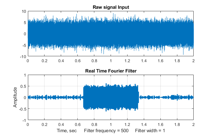 compute
each filtered
section.
"WindowWidth" (line 55) is the number
of data points in each segment. The larger this number, the
fewer the number of segments that will
be generated, but the higher will be
the frequency resolution within each
segment. On a standard desktop PC
(Intel Core i5 3 Ghz running Windows
10 home), with a window width of 1000
points, this script generates about 35
filtered segments per second with an
average data rate (points per second)
of about 34,000 Hz. Smaller segments
(i.e. lower values of WindowWidth)
generate proportionally lower average
data rate (because the signal stream
is interrupted more often to calculate
and graph the filtered spectrum). The
result of applying the filter to each
segment is displayed in real time
during the data acquisition, and then
at the end the script compares the
entire raw signal input to the
reassembled filtered output, shown the
the figure on the left.
compute
each filtered
section.
"WindowWidth" (line 55) is the number
of data points in each segment. The larger this number, the
fewer the number of segments that will
be generated, but the higher will be
the frequency resolution within each
segment. On a standard desktop PC
(Intel Core i5 3 Ghz running Windows
10 home), with a window width of 1000
points, this script generates about 35
filtered segments per second with an
average data rate (points per second)
of about 34,000 Hz. Smaller segments
(i.e. lower values of WindowWidth)
generate proportionally lower average
data rate (because the signal stream
is interrupted more often to calculate
and graph the filtered spectrum). The
result of applying the filter to each
segment is displayed in real time
during the data acquisition, and then
at the end the script compares the
entire raw signal input to the
reassembled filtered output, shown the
the figure on the left.
In this demonstration, a bandpass
filter is used to detect a 500 Hz sine
wave (the
frequency is controlled by 'f' in line
28) that occurs in the middle third of
a very noisy signal (line 32), from
about 0.7 sec to 1.3 sec. The 500
Hz sine wave
is so weak it
can not be
seen at all in
the raw signal
(upper panel
of the figure
on the left).
The
filter center frequency
(CenterFrequency) and width
(FilterWidth) are set in lines 46 and
47.
Real-time classical least squares.
The classical
least squares technique can be
applied in real time to 2D
chromatography with array detectors
that can acquire a complete spectrum
multiple times per second over the
entire chromatogram. This is explored
in "Spectroscopy
and chromatography combined:
time-resolved Classical Least
Squares".
To apply any of these examples
to real-time data from your sensor or
instrument, you need only the main
processing 'for' loop, replacing the
first lines after the 'for' statement
with a call to a function that
acquires a single point of raw data
and assigns it to y(n). If you don't
need the data plotted out
point-by-point in real time, you can
speed things up greatly by removing
the "drawnow" statement at the end of
the 'for' loop or by removing all the
plotting code.
In the examples here, the output of the
processing operation is used to plot or to print out the processed
data point-by-point, but of course it could also be used as the
input to another processing function or to a digital-to-analog converter or simply to
trigger an alarm if certain specified results are obtained (e.g.
if the signal exceeds a certain value for a specified length of
time, or if a peak is detected at a specified position or height,
etc).
This page is part of "A Pragmatic Introduction to Signal
Processing", created and maintained by Prof. Tom O'Haver ,
Department of Chemistry and Biochemistry, The University of Maryland
at College Park. Comments, suggestions and questions should be
directed to Prof. O'Haver at toh@umd.edu. Updated July, 2022.