These are fill-in-the-blanks spreadsheet templates for performing
the calibration curve
fitting and concentration calculations for analytical methods
using the calibration curve method. All you have to do is to
type in (or paste in) the concentrations of the standard solutions
and their instrument readings (e.g. absorbances, or whatever method
you are using) and the instrument readings of the unknowns. The
spreadsheet automatically plots and fits the data to a straight
line, quadratic or cubic curve, then uses the equation of that curve
to convert the readings of the unknown samples into concentration.
You can add and delete calibration points at will, to correct
errors or to remove outliers; the sheet re-plots and recalculates
automatically.
Screen shots and Download
links:
Linear
calibration
with error calculation.
Download Excel or
OpenOffice Calc
format.
Linear interpolation
(bracket method). Download Excel or
OpenOffice Calc
format
Quadratic calibration
with error estimation.
Download Excel
or OpenOffice Calc
format
Cubic calibration. Download Excel or OpenOffice Calc format.
Log-log calibration. Download
log-log linear (.xls
or .ods) or
log-log quadratic (.xls or .ods)
Drift-corrected
quadratic calibration. Download Excel or
OpenOffice Calc
format.
Note: to run these
spreadsheets, you must have either Excel or OpenOffice Calc
installed. I recommend either Excel 2013 or OpenOffice Version
4 (download
from OpenOffice).
In analytical chemistry, the accurate quantitative measurement of
the composition of samples, for example by various types of
spectroscopy, usually requires that the method be calibrated
using standard samples of known composition. This is most
commonly, but not necessarily, done with solution samples and
standards dissolved in a suitable solvent, because of the ease of
preparing and diluting accurate and homogeneous mixtures of
samples and standards in solution form. In the calibration curve
method, a series of external standard solutions is prepared and
measured. A line or curve is fit to the data and the resulting
equation is used to convert readings of the unknown samples into
concentration. An advantage of this method is that the random
errors in preparing and reading the standard solutions are
averaged over several standards. Moreover, non-linearity in the
calibration curve can be detected and avoided (by diluting into
the linear range) or compensated (by using non-linear curve
fitting methods). There are worksheets here for several different
calibration methods:
A first-order (straight line)
fit of measured signal A (y-axis) vs concentration C (x-axis). The model
equation is A
=slope * C
+ intercept. This is
the most common and straightforward method, and it is the one to
use if you know that
your instrument response is linear. This fit is performed using
the equations described and listed on http://terpconnect.umd.edu/~toh/spectrum/CurveFitting.html.
You need a minimum of two
points on the calibration curve. The concentration of unknown
samples is given by (A - intercept) / slope where A is the
measured signal and slope
and intercept from the
first-order fit. If you would like to use this method of
calibration for your own data, download in Excel or OpenOffice Calc format. View
equations for linear
least-squares.
Linear interpolation calibration.In the linear interpolation method (sometime called
the bracket method), the spreadsheet performs a linear
interpolation between the two standards that are just
above and just below each unknown sample, rather than doing
a least-squares fit over then entire calibration set. The
concentration of the sample Cx is calculated by
C1s+(C2s-C1s)*(Sx-S1s)/(S2s-S1s), where S1x and S2s are the
signal readings given by the two standards that
are just above and just below the unknown sample,
C1s and C2s are the
concentrations of those two standard solutions,
and Sx is the signal given by the sample solution. This
method may be useful if none
of the least-squares methods are capable of fitting the
entire calibration range adequately (for
instance, if it contains two linear segments with different
slopes). It works well enough as long as the standards are
spaced closely enough so that the actual signal response
does not deviate significantly from linearity between the
standards. However, this method does not deal well with
random scatter in the calibration data due to random noise,
because it does not compute a "best-fit" through multiple
calibration points as the least-squares methods do. Download
a template in Excel
(.xls) format.
A quadratic fit of
measured signal A
(y-axis) vs concentration C
(x-axis). The model equation is A
= aC2 + bC + c.
This method can compensate for non-linearity in the instrument
response to concentration. This fit is performed using the
equations described and listed on http://terpconnect.umd.edu/~toh/spectrum/CurveFitting.html.
You need a minimum of three
points on the calibration curve. The concentration of unknown
samples is calculated by solving this equation for C using the classical
"quadratic formula", namely
C = (-b+SQRT(b2-4*a*(c-A)))/(2*a),
whereA = measured signal,
and a, b, and c are the three
coefficients from the quadratic fit. If you would like to
use this method of calibration for your own data, download
in Excel or
OpenOffice Calc
format. View equations for quadratic least-squares.
The alternative version CalibrationQuadraticB.xlsx
computes the concentration standard deviation (column L)
and percent relative standard deviation (column M) using
the bootstrap
method. You need at least 5 standards for the error
calculation to work. If you get a "#NUM!" or #DIV/0" in
the columns L or M, just press the F9 key
to re-calculate the spreadsheet. There is also a reversed quadratic
template and example,
which is analogous to the reversed cubic (#5 below).
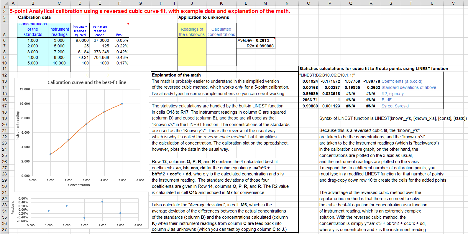
A reversed cubic fit
of concentration C
(y-axis) vs measured signal A (x-axis). The model equation isC = aA3 + bA2 + cA + d. This method can
compensate for more complex non-linearity that the quadratic
fit. A "reversed fit" flips the usual order of axes, by
fitting concentration as a function of measured signal. This is
done in order to avoid the need to solve a
cubic equation when the calibration equation is solved
for C and used to convert the measured signals of the unknowns
into concentration. This coordinate transformation is a
short-cut, commonly done in least-squares curve fitting, at
least by non-statisticians, to avoid
mathematical messiness when the fitting equation is solved for
concentration and used to convert the instrument readings into
concentration values. However, this method is theoretically not
optimum, as demonstrated for the quadratic case Monte-Carlo
simulation in
the spreadsheet NormalVsReversedQuadFit2.ods(Screen
shot),
and should be used only if the experimental calibration curve is
so non-linear that it can not be fit at all by a quadratic - #3
above.
This reversed cubic fit is performed using the LINEST
function on Sheet3. You need a minimum of four points on the
calibration curve. The concentration of unknown samples is
calculated directly by aA3+bA2+c*A+d, whereA is the
measured signal, and a,
b, c, and d are the four coefficients
from the cubic fit. The math is shown and explained better
in the template CalibrationCubic5Points.xls
(screen image), which
is set up for a 5-point calibration, with sample data already
entered. To expand this template to a greater number of
calibration points, follow these steps exactly: select row 9
(click on the "9" row label), right-click and select Insert,
and repeat for each additional calibration point required. Then
select row 8 columns D through K and
drag-copy them down to fill in the newly created rows.
That will create all the required equations and will modify the
LINEST function in O16-R20. There is also another template, CalibrationCubic.xls, that uses
some spreadsheet "tricks" to automatically sense the
number of calibration points you enter and adjust the
calculations accordingly; download in Excel or OpenOffice Calc format.
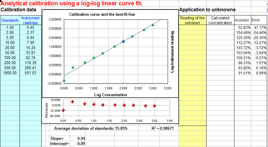
Log-log Calibration.In log-log
calibration, the logarithm of the measured signal A (y-axis) is plotted
against the logarithm of concentration C (x-axis) and the
calibration data are fit to a linear or quadratic model, as in
#1 and #2 above. The concentration of unknown samples is
obtained by taking the logarithm of the instrument readings,
computing the corresponding logarithms of the concentrations
from the calibration equation, then taking the anti-log to
obtain the concentration. (These additional steps do not
introduce any additional error, because the log and anti-log
conversions can be made quickly and without significant error by
the computer). Log-log calibration is well suited for data with
very large range of values because it distributes the relative
fitting error more evenly among the calibration points,
preventing the larger calibration points to dominate and cause
excessive errors in the low points. In some cases (e.g Power Law
relationships) a nonlinear relationship between signal and
concentration can be completely linearized by a
log-log transformation. However,
because of the use of logarithms, the data set can not contain
any zero or negative values. To use this method of
calibration for your own data, download
the templates for log-log linear (Excel or Calc) or log-log
quadratic (Excel or Calc).
Drift-corrected calibration. All of the above methods assume that the
calibration of the instrument is stable with time and that the
calibration (usually performed before the samples are measured)
remains valid while the unknown samples are measured. In
some cases, however, instruments and sensors can drift, that is, the slope
and/or intercept of their calibration curves can gradually
change with time after the initial calibration. You can test for
this drift by measuring the standards again after the samples are run,
to determine how different the second calibration curve is from
the first. If the difference is not too large, it's reasonable
to assume that the drift is approximately linear with time, that
is, that the calibration curve parameters (intercept, slope, and
curvature) have changed linearly as a function of time between
the two calibration runs. It's then possible to correct
for the drift if you record the time when each calibration is run and when
each unknown sample is measured. The drift-correction
spreadsheet (CalibrationDriftingQuadratic.ods) does the
calculations: it computes a quadratic fit for the pre- and
post-calibration curves, then uses linear interpolation to
estimate the calibration curve parameters for each separate
sample based on the time it was measured. The method works
perfectly only if the drift is linear with time (a reasonable
assumption if the amount of drift is not too large), but in any
case it is better than simply assuming that there is no drift at
all. If you would like to use this method of calibration for
your own data, download in Excel or
OpenOffice Calc
format. (See Instructions:
#8).
Error calculations. In many cases it is important to
calculate the likely error in the computed concentration values
(column K) caused by imperfect calibration. This is discussed on
"Reliability
of curve fitting results". The linear calibration
spreadsheet (download in Excel or OpenOffice Calc format) performs a
classical algebraic error-propagation calculation on the
equation that calculates the concentration from the unknown
signal and the slope and intercept of the calibration curve.
The quadratic calibration
spreadsheet (Download
in Excel
or OpenOffice Calc
format) performs a bootstrap
calculation. You must have a least 5
calibration points for these error calculations to be even
minimally reliable; the more the better. That is because
these methods need a representative sample of deviations
from the ideal calibration line. If the calibration line
fits the points exactly, then the computed error will be
zero.
Instructions:
1. Download and open the desired calibration worksheet
from among those listed
above.
2. Enter the concentrations of the standards and their instrument
readings (e.g. absorbance) into the blue table on the left. Leave
the rest of the table blank. You must have at least two points on
the calibration curve (three points for the quadratic method or four
points for the cubic method), including the blank (zero
concentration standard). If you have multiple instrument readings
for one standard, it's better to enter each as a separate standard
with the same concentration, rather than entering the average. The
spreadsheet automatically gives more weight to standards that have
more than one reading.
3. Enter the instrument readings (e.g. absorbance) of the unknowns
into the yellow table on the right. You can have any number of
unknowns up to 20. (If you have multiple instrument readings for one
unknown, it's better to enter each as a separate unknown, rather
than averaging them, so you can see how much variation in calculated
concentration is produced by the variation in instrument
reading).
4. The concentrations of the unknowns are automatically calculated
and displayed column K. If you edit the calibration curve, by
deleting, changing, or adding more calibration standards, the
concentrations are automatically recalculated.
For the linear fit (CalibrationLinear.xls), if you have three or
more calibration points, the estimated standard deviation of the
slope and intercept will be calculated and displayed in cells G36
and G37, and the resulting standard deviation (SD) of each
concentration will be displayed in rows L (absolute SD) and M
(percent relative SD). These standard deviation calculations are
estimates of the variability of slopes and intercepts you are likely
to get if you repeated the calibration over and over multiple times
under the same conditions, assuming that the deviations from the
straight line are due to random variability and not
systematic error caused by non-linearity. If the deviations are
random, they will be slightly different from time to time, causing
the slope and intercept to vary from measurement to measurement..
However, if the deviations are caused by systematic non-linearity,
they will be the same from from measurement to measurement, in which
case these predictions of standard deviation will not be relevant,
and you would be better off using a.polynomial fit such as a
quadratic or cubic. The reliability of these standard deviation
estimates also depends on the number of data points in the curve
fit; they improve with the square root of the number of points.
5. You can remove any point from the curve fit by deleting the
corresponding X and Y values in the table. To delete a value;
right-click on the cell and click "Delete Contents" or "Clear
Contents". The spreadsheet automatically re-calculates and the graph
re-draws; if it does not, press F9 to recalculate. (Note: the cubic
calibration spreadsheet must have contiguous calibration points with
no blank or empty cells in the calibration range).
6. The linear calibration spreadsheet also calculates the
coefficient of determination, R2, which is an indicator
of the "goodness of fit", in cell C37. R2 is 1.0000
when the fit is perfect but less than that when the fit is
imperfect. The closer to 1.0000 the better.
7. A "residuals plot" is displayed just below the calibration graph
(except for the interpolation method). This shows the
difference between the best-fit calibration curve and the actual
readings of the standards. The smaller these errors, the more
closely the curve fits the calibration standards. (The
standard deviation of those errors is also calculated and displayed
below the residuals plot; the lower this standard deviation, the
better).
You can tell a lot by looking at the shape of the residual plot: if
the points are scattered randomly above and below zero, it
means that the curve fit is as
good as it can be given the random noise in the data.
But if the residual plot has a smooth shape, say, a U-shaped
curve, then it means that there is a mismatch between the curve fit
and the actual shape of the calibration curve; suggesting that the
another curve fitting techniques might be tried (say, a quadratic or
cubic fit rather than a linear one) or that the experimental
conditions be modified to produce a less complex experimental
calibration curve shape.
8. If you are using the spreadsheet for drift-corrected calibration,
you must measure two
calibration curves, one before
and one after the samples
are run, and record the date and time each calibration curve is
measured. Enter the concentrations of the standards into
column B. Enter the
instruments readings for the first (pre-) calibration into column C and the date/time of that
calibration into cell C5;
enter the instruments readings for the post-calibration into column
D and the date/time of that
calibration into cell D5.
The format for the date/time entry is Month-Day-Year Hours:Minutes:Seconds, for example
6-2-2011 13:30:00 for June 2, 2011, 1:30 PM (13:30 on the 24-hour
clock). Note: if both calibrations are run on the same day,
you can leave off the date and just enter the time. In the
graph, the pre-calibration curve is shown in green and the
post-calibration curve is shown in red.
Then, for each unknown sample measured, enter the date/time (in the
same format) into column K
and the instrument reading for that unknown into column L. The spreadsheet computes the
drift-corrected sample concentrations in column M. Note: Version 2.1 of this
spreadsheet (July, 2011) allows different sets of concentrations for
the pre- and post-calibrations. Just list all he concentrations used
in the "Concentration of standards" column (B) and put the
corresponding instrument readings in columns C or D, or both. If you don't use a
particular concentration for one of the calibrations, just leave
that instrument reading blank.
Click to see larger
figure
This figure shows an application of the drift-corrected quadratic
calibration spreadsheet. In this demonstration, the calibrations and
measurements were made over a period of several days. The
pre-calibration (column C)
was performed with six standards (column B) on 01/25/2011 at 1:00 PM. Eight unknown samples
were measured over the following five days (columns L and M), and the post-calibration (column D) was performed after then last
measurement on 01/30/2011 at 2:45 PM. The graph in the center
shows the pre-calibration curve in green and the post-calibration
curve in red. As you can see, the sensor (or the instrument) had
drifted over that time period, the sensitivity (slope of the
calibration curve) becoming smaller and curve becoming noticeably
more non-linear (concave down). However, both the pre- and
post-calibration curves fit the quadratic calibration equations very
well, as indicated by the residuals plot and the coefficients of
determination (R2) listed
below the graphs. The eight "unknown" samples that were measured for
this test (yellow table) were actually the same sample measured
repeatedly - a standard of concentration 1.00 units - but you can
see that the sample gave lower instrument readings (column L) each time it was measured
(column K), due to the
drift. Finally, the drift-corrected concentrations calculated
by the spreadsheet (column M
on the right) are all very close to 1.00, showing that the drift
correction works well, within the limits of the random noise in the
instrument readings and subject to the assumption that the drift in
the calibration curve parameters is linear with time between the
pre- and post-calibrations.
Frequently Asked Questions (taken
from actual search engine queries)
1. Question:What is the the purpose of calibration
curve? Answer: Most
analytical instruments generate an electrical output signal such as
a current or a voltage. A calibration curve establishes the
relationship between the signal generated by a measurement
instrument and the concentration of the substance being measured.
Different chemical compounds and elements give different signals.
When an unknown sample is measured, the signal from the unknown is
converted into concentration using the calibration curve.
2. Question:How
do you make a calibration curve? Answer: You prepare a
series of "standard solutions" of the substance that you intend to
measure, measure the signal (e.g. absorbance, if you are doing
absorption spectrophotometry), and plot the concentration on the
x-axis and the measured signal for each standard on the y-axis. Draw
a straight line as close as possible to the points on the
calibration curve (or a smooth curve if a straight line won't fit),
so that as many points as possible are right on or close to the
curve.
3. Question:How do
you use a calibration curve to predict the concentration of an
unknown sample? How do you determine concentration from a
non-linear calibration plot? Answer: This can be
done in two ways, graphically and mathematically. Graphically, draw
a horizontal line from the signal of the unknown on the y axis over to the calibration
curve and then straight down to the concentration (x) axis to the concentration of
the unknown. Mathematically, fit an equation to the calibration
data, and solve the equation for concentration as a function of
signal. Then, for each unknown, just plug its signal into this
equation and calculate the concentration. For example, for a linear
equation, the curve fit equation is Signal =slope
* Concentration + intercept, where slope and intercept are determined by a
linear (first order) least
squares curve fit to the calibration data. Solving this
equation for Concentration
yields Concentration = (Signal-
intercept) / slope,
where Signal is the signal
reading (e.g. absorbance) of the unknown solution. (Click
here for a fill-in-the-blank OpenOffice spreadsheet that
does this for you.
View
screen shot).
4. Question:How
do I know when to use a straight-line curve fit and when to use a
curved line fit like a quadratic or cubic? Answer: Fit a straight line to the
calibration data and look at a plot of the "residuals"
(the differences between the y
values in the original data and the y values computed by the fit equation).Deviations from linearity will be
much more evident in the residuals plot than in the calibration
curve plot.(Click
here for a fill-in-the-blank OpenOffice spreadsheet that
does this for you.
View
screen shot). If the residuals are randomly scattered all
along the best-fit line, then it means that the deviations are
caused by random errors such as instrument noise or by random
volumetric or procedural errors; in that case you can use a
straight line (linear) fit. If the residuals have a
smooth shape, like a "U" shape, this means that the
calibration curve is curved, and you should use a non-linear
curve fit, such as a quadratic
or cubic fit. If the residual plot has a "S" shape,
you should probably use a cubic fit. (If you are doing
absorption spectrophotometry, see Comparison of Curve Fitting Methods
in Absorption Spectroscopy).
5. Question:What
if my calibration curve is linear at low concentrations but curves
off at the highest concentrations? Answer: You can't use
a linear curve fit in that case, but if the curvature is not too
severe, you might be able to get a good fit with a quadratic or cubic fit.
If not, you could break the concentration range into two
regions and fit a linear curve to the lower linear region
and a quadratic or cubic curve to the higher non-linear region.
6. Question:What
is the difference between a calibration curve and a line of best
fit? What is the difference between a linear fit and a
calibration curve. Answer: The
calibration curve is an experimentally measured relationship between
concentration and signal. You don't ever really know the true calibration curve; you can
only estimate it at a few
points by measuring a series of standard solutions. Then draw a line
or a smooth curve that goes as much as possible through the points,
with some points being a little higher than the line and some points
a little lower than the line. That's what we mean by that is a "best
fit" to the data points. The actual calibration curve might
not be perfectly linear, so a linear fit is not always the best.
A quadratic or cubic fit might be better if the calibration
curve shows a gradual smooth curvature.
7. Question:Why
does the slope line not go through all points on a graph? Answer: That will only
happen if you (1) are a perfect experimenter, (2) have a perfect
instrument, and (3) choose the perfect curve-fit equation for your
data. That's not going to happen. There are always little errors. The
least-squares curve-fitting method yields a best fit, not a perfect fit, to the calibration
data for a given curve shape (linear. quadratic, or cubic). Points
that fall off the curve are assumed to do so because of random
errors or because the actual calibration curve shape does not match
the curve-fit equation.
Actually, there is one artificial way you can make the curve go
through all the points, and that is to use too few calibration standards: for example, if you
use only two points for a
straight-line fit, then the best-fit line will go right through
those two points no matter what.
Similarly, if you use only three points for a quadratic fit, then the
quadratic best-fit curve will go right through those three points,
and if you use only four
points for a cubic fit, then the cubic best-fit curve will go
right through those four points. But that's not really
recommended, because if one of your calibration points is really off
by a huge error, the curve fit willstill look perfect, and
you'll have no clue that
something's wrong. You really have to use more standards that that
so that you'll know when something has gone wrong.
8. Question:What
happens when the absorbance reading is higher than any of the
standard solutions? Answer: If you're
using a curve-fit equation, you'll still get a value of
concentration calculated for any
signal reading you put in, even above the highest standard.
However, it's risky to do that, because you really don't know
for sure what the shape of the calibration curve is above the
highest standard. It could continue straight or it could curve off
in some unexpected way - how would you know for sure? It's
best to add another standard at the high end of the calibration
curve.
9. Question:What's
the difference between using a single standard vs multiple
standards and a graph? Answer: The single
standard method is the simplest and quickest method, but it is
accurate only if the calibration curve is known to be linear. Using
multiple standards has the advantage that any non-linearity in the
calibration curve can be detected and avoided (by diluting into the
linear range) or compensated (by using non-linear curve fitting
methods). Also, the random errors in preparing and reading the
standard solutions are averaged over several standards, which is
better than "putting all your eggs in one basket" with a single
standard. On the other hand, an obvious disadvantage of the
multiple standard method is that it requires much more time and uses
more standard material than the single standard method.
10. Question:What's
the relationship between sensitivity in analysis and the slope of
standard curve? Answer: Sensitivity is
defined as the
slope of the standard (calibration) curve.
11. Question:How do
you make a calibration curve in Excel or in OpenOffice? Answer: Put the
concentration of the standards in one column and their signals (e.g.
absorbances) in another column. Then make an XY scatter
graph, putting concentration on the X (horizontal) axis and
signal on the Y (vertical) axis. Plot the data points with
symbols only, not lines between the points. To compute a
least-squares curve fit, you can either put in the least-squares
equations into your spreadsheet, or you can use the built-in
LINEST function in both Excel
and OpenOffice
Calc to compute polynomial and other curvilinear least-squares
fits. For examples of OpenOffice spreadsheets that graphs and
fits calibration curves, see Worksheets for Analytical Calibration
Curves. 12. Question:What's
the
difference in using a calibration curve in absorption spectrometry
vs other analytical methods such a fluorescence or emission
spectroscopy? Answer: The only
difference is the units of the signal. In absorption spectroscopy
you use absorbance
(because it's the most nearly linear with concentration) and in
fluorescence (or emission) spectroscopy you use the fluorescence (or emission) intensity,
which is usually linear with concentration (except sometimes at high
concentrations). The methods of curve fitting and calculating the
concentration are basically the same.
13. Question:If
the solution obeys Beer's Law, is it better to use a calibration
curve rather than a single standard? Answer: It might not
make much difference either way. If the solution is known from
previous measurements to obey Beer's Law exactly on the same
spectrophotometer and under the conditions in use, then a single
standard can be used (although it's best if that standard gives a
signal close to the maximum expected sample signal or to whatever
signal gives the best signal-to-noise ratio - an absorbance near 1.0
in absorption spectroscopy). The only real advantage of multiple
standards in this case is that the random errors in preparing and
reading the standard solutions are averaged over several standards,
but the same effect can be achieved more simply by making up
multiple copies of the same single standard (to average out the
random volumetric errors) and reading each separately (to average
out the random signal reading errors). And if the signal
reading errors are much smaller than the volumetric errors, then a single standard solution can be
measured repeatedly to average out the random measurement errors.
14. Question:What
is the effect on concentration measurement if the monochromator is
not perfect? Answer: If the
wavelength calibration if off a little bit, it will have no
significant effect as long as the monochromator setting is left
untouched between measurement of standards and unknown sample; the
slope of the calibration curve will be different, but the calculated
concentrations will be OK. (But if anything changes the
wavelength between the time you measure the standards and the time
you measure the samples, an error will result). If the wavelength
has a poor stray light rating or if the resolution is poor (spectral
bandpass is too big), the calibration curve may be effected
adversely. In absorption spectroscopy, stray light and poor
resolution may result in non-linearity, which requires a non-linear
curve fitting method. In emission spectroscopy, stray light and poor
resolution may result in a spectral interferences which can result
in significant analytical errors.
15. Question:What
does it mean if the intercept of my calibration curve fit is not
zero? Answer: Ideally the
y-axis intercept of the calibration curve (the signal at zero
concentration) should be zero, but there are several reasons why
this might not be so. (1) If there is substantial random
scatter in the calibration points above and below the best-fit line,
then it's likely that the non-zero intercept is just due to random
error. If you prepared another separate set of standards, that
standard curve would have different intercept, either positive or
negative. There is nothing that you can do about this, unless you
can reduce the random error of the standards and samples. (2) If the
shape of the calibration curve does not match the shape of the curve
fit, then it's very likely that you'll get a non-zero intercept
every time. For example, if the calibration curve bends down as
concentration increases, and you use a straight-line (linear) curve
fit, the intercept will be positive (that is, the curve fit line
will have a positive y-axis intercept, even if the actual
calibration curve goes through zero). This is an artifact of the
poor curve fit selection; if you see that happen, try a different
curve shape (quadratic or cubic). (3) If the instrument is not
"zeroed" correctly, in other words, if the instrument gives a
non-zero reading when the blank
solution is measured. In that case you have three choices: you
can zero the instrument (if that's possible); you can subtract the
blank signal from all the standard and sample readings; or you can
just let the curve fit subtract the intercept for you (if your curve
fit procedure calculates the intercept and you keep it in the
solution to that equation, e.g. Concentration = (Signal - intercept) / slope).
16. Question:How
can I reduce the random scatter of calibration points above and
below the best-fit line? Answer: Random errors
like this could be due either to random volumetric errors (small
errors in volumes used to prepare the standard solution by diluting
from the stack solution or in adding reagents) or they may be due to
random signal reading errors of the instrument, or to both. To
reduce the volumetric error, use more precise volumetric equipment
and practice your technique to perfect it (for example, use your
technique to deliver pure water and weigh it on a precise analytical
balance). To reduce the signal reading error, adjust the instrument
conditions (e.g. wavelength, path length, slit width,
etc) for best signal-to-noise ratio and average several
readings of each sample or standard.
17. Question:What
are
interferences? What effect do interferences have on the
calibration curve and on the accuracy of concentration
measurement? Answer: When an
analytical method is applied to complex real-world samples, for
example the determination of drugs in blood serum, measurement error
can occur due to interferences.
Interferences are measurement errors caused by chemical components in the samples
that influence the measured signal, for example by contributing
their own signals or by reducing or increasing the signal from the
analyte. Even if the method is well calibrated and is capable of
measuring solutions of pure analyte accurately, interference errors may occur when the method is
applied to complex real-world samples. One way to correct for
interferences is to use "matched-matrix standards", standard
solution that are prepared to contain everything that the real samples contain, except
that they have known concentrations of analyte. But this is very
difficult and expensive to do exactly, so every effort is made to
reduce or compensate for interferences in other ways. For more
information on types of interferences and methods to compensate
for them, see Comparison of
Analytical Calibration Methods.
18. Question:What are the sources of error in
preparing a calibration curve? Answer: A calibration
curve is a plot of analytical signal (e.g. absorbance, in absorption
spectrophotometry) vs concentration of the standard solutions.
Therefore, the main sources of error are the errors in the standard
concentrations and the errors in their measured signals.
Concentration errors depend mainly of the accuracy of the volumetric
glassware (volumetric flasks, pipettes, solution delivery devices)
and on the precision of their use by the persons preparing the
solutions. In general, the accuracy and precision of handling
large volumes above 10 mL is greater than that at lower volumes
below 1 mL. Volumetric glassware can be calibrated by weighing water
on a precise analytical balance (you can look up the density of
water at various temperatures and thus calculate the exact volume of
water from its measured weight); this would allow you to label each
of the flasks, etc, with their actual volume. But precision may
still be a problem, especially a lower volumes, and it's very much
operator-dependent. It takes practice to get good at handling small
volumes. Signal measurement error depends hugely on the instrumental
method used and on the concentration of the analyte; it can vary
from near 0.1% under ideal conditions to 30% near the detection
limit of the method. Averaging repeat measurements can improve
the precision with respect to random noise. To improve the
signal-to-noise ratio at low concentrations, you may consider
modifying the conditions, such as changing the slit width or the
path length, or using another instrumental method (such as a
graphite furnace atomizer rather than flame atomic absorption).
19. How can I find the error in a specific
quantity using least square fitting method? How can I estimate the error in the
calculated slope and intercept?
When using a simple straight-line (first order) least-squares fit,
the best fit line is specified by only two quantities: the slope and the intercept. The random error in the slope and
intercept (specifically, their standard deviation) can
be estimated mathematically from the extent to which the calibration
points deviate from the best-fit line. The equations for doing this
are given here and are
implemented in the "spreadsheet
for linear
calibration with error calculation".
It's important to realize
that these error computations are only estimates, because
they are based on the assumption that the calibration data set is
representative of all the calibration sets that would be obtained if
you repeated the calibration a large number of times - in other
words, the assumption is that the random errors (volumetric and
signal measurement errors) in your particular data set are typical.
If your random errors happen to be small when you run your
calibration curve, you'll get a deceptively good-looking calibration curve,
but your estimates of the random error in the slope and intercept
will be too low. If
your random errors happen to be large, you'll get a deceptively bad-looking calibration curve,
and your estimates of the random error in the slope and intercept
will be too high. These
error estimates can be particularly poor when the number of points
in a calibration curve is small; the accuracy of the estimates
increases if the number of data points increases, but of course
preparing a large number of standard solutions is time consuming and
expensive. The bottom line is that you can only expect these
error predictions from a single calibration curve to be very rough;
they could easily be off by a factor of two or more, as demonstrated
by the simulation "Error propagation in the Linear Calibration Curve
Method" (download
OpenOffice version).
20. How can I estimate the error in the
calculated concentrations of the unknowns?
You can use the slope and intercept from the least-squares fit to calculate the
concentration of an unknown solution by measuring its signal and
computing (Signal- intercept) /
slope, where Signal is the signal reading
(e.g. absorbance) of the unknown solution. The errors in this
calculated concentration can then be estimated by the usual rules
for the propagation of error: first, the error in (Signal- intercept) is computed by the rule for addition
and subtraction; second, the error in (Signal- intercept) /
slope is computed
by the rule for multiplication and division. The equations for doing
this are given here and are
implemented in the "spreadsheet
for linear
calibration with error calculation".
It's important to realize
that these error computations are only estimates, for the
reason given in #19 above, especially if the number of points in a
calibration curve is small, as demonstrated by the simulation "Error
propagation in the Linear Calibration Curve Method" (download OpenOffice version).
21.What is the minimumacceptable value of the
coefficient of determination (R2)?
It depends on the accuracy required. As a rough rule of thumb,
if you need an accuracy of about 0.5%, you need an R2
of 0.9998; if a 1% error is good enough, an R2 of 0.997 will do; and if a 5%
error is acceptable, an R2 of 0.97 will do. The bottom line
is that the R2 must be pretty darned close to
1.0 for quantitative results in analytical chemistry. (c) 2008, 2021 Prof.
Tom
O'Haver , Professor Emeritus, The University of Maryland at
College Park. Comments, suggestions and questions should be directed
to Prof. O'Haver at toh@umd.edu.
Number of unique visits since May
17, 2008. Last updated October, 2021


