In the section
of Signals
and Noise, I said: "The quality of a signal is often
expressed as the signal-to-noise (S/N) ratio, which is the ratio
of the true signal amplitude ... to the standard deviation of
the noise." That's a simple enough statement, but automating the
measurement of signal and the noise in real signals is not
always straightforward. Sometimes it's difficult to separate or
distinguish between the signal and the noise, because it depends
not only on the numerical nature of the data, but also on the
objectives of the measurement.
For a simple DC (direct current) signal, for example measuring a
fluctuating voltage, the signal is just the average voltage
value and the noise is its standard deviation. This is easily
calculated in a spreadsheet or in Matlab/Octave:
>>
signal=mean(NoisyVoltage);
>> noise=std(NoisyVoltage);
>> SignalToNoiseRatio=signal/noise
 But
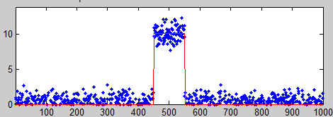
usually things are more complicated. For example, if the signal
is a rectangular pulse (as in the figure on the left) with
constant random noise, then the simple formulation above will
not give accurate results. If the signal is stable enough that
you can get two successive signal recordings m1 and m2 that are identical except for the noise, then you can simply
subtract the signal out: the
standard deviation of the noise is then given by sqrt((std(m1-m2)2)/2), where std is the standard
deviation function (because random noise
adds quadratically). But not every signal source is stable
and repeatable enough for that to work perfectly. Alternatively,
you can try to measure the average signal just over the top of
the pulse and the noise only over the baseline interval before
and/or after the pulse. That's not so hard to do by hand, but
it's harder to automate with a computer, especially if the
position or width of the pulse changes. It's basically the same
for smooth peak shapes like the commonly-encountered Gaussian
peak (as in the figure on the right)
But
usually things are more complicated. For example, if the signal
is a rectangular pulse (as in the figure on the left) with
constant random noise, then the simple formulation above will
not give accurate results. If the signal is stable enough that
you can get two successive signal recordings m1 and m2 that are identical except for the noise, then you can simply
subtract the signal out: the
standard deviation of the noise is then given by sqrt((std(m1-m2)2)/2), where std is the standard
deviation function (because random noise
adds quadratically). But not every signal source is stable
and repeatable enough for that to work perfectly. Alternatively,
you can try to measure the average signal just over the top of
the pulse and the noise only over the baseline interval before
and/or after the pulse. That's not so hard to do by hand, but
it's harder to automate with a computer, especially if the
position or width of the pulse changes. It's basically the same
for smooth peak shapes like the commonly-encountered Gaussian
peak (as in the figure on the right)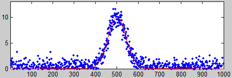 . You can estimate the
height of the peak by smoothing it and then taking the
maximum of the smoothed peak as the signal: max(fastsmooth(y,10,3)), but the accuracy would degrade if you choose too high
or two low a smooth width. And clearly all this depends on
having a well-defined baseline in the data where there is only
noise. It doesn't work if the noise varies with the amplitude of
the peak.
. You can estimate the
height of the peak by smoothing it and then taking the
maximum of the smoothed peak as the signal: max(fastsmooth(y,10,3)), but the accuracy would degrade if you choose too high
or two low a smooth width. And clearly all this depends on
having a well-defined baseline in the data where there is only
noise. It doesn't work if the noise varies with the amplitude of
the peak.
In many cases, curve fitting can be helpful. For example, you could use peak fitting or a peak detector to locate multiple peaks and measure their peak heights and their S/N ratios on a peak-to-peak basis, by computing the noise as the standard deviation of difference between the raw data and the best-fit line over the top part of the peak. That's how iSignal measures S/N ratios of peaks. Also, iSignal has baseline correction capabilities that allow the peak to be measured relative to the nearby baseline.
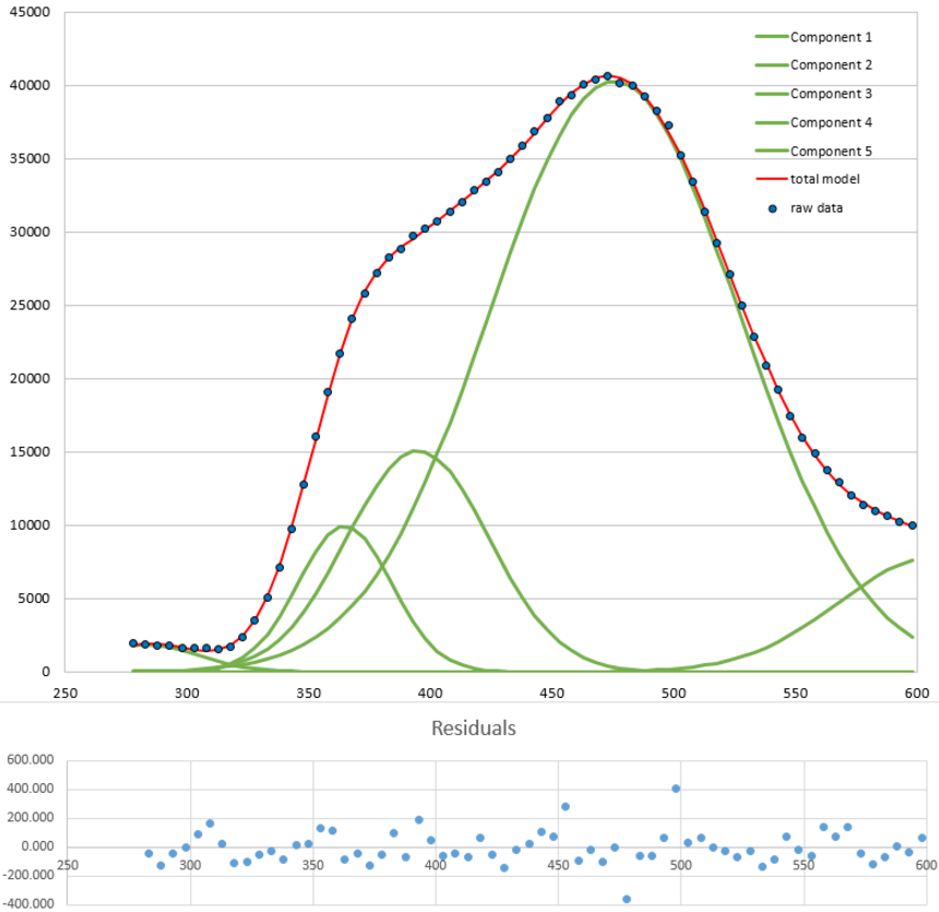 Curve
fitting also works for complex signals of indeterminate shape
that can be approximated by a high-order
polynomial or as the sum
of a number of basic functions such as Gaussians, as in
the example shown on the left. In this example, five Gaussians
are used to fit the data to the point where the residuals are
random and unstructured. The residuals (shown in blue below the
graph) are then just the noise remaining in the signal, whose
standard deviation is easily computed using the built-in standard deviation
function in a spreadsheet ("STDEV") or in Matlab/Octave ("std").
In this example, the standard deviation of the residuals is 111
and the maximum signal is 40748, so the percent relative
standard deviation of the noise is 0.27% and the S/N ratio is
367. (The positions, heights, and widths of the Gaussian
components, usually the main results of the curve fitting, are
not used in this case; curve fitting is used only to obtain a
measure the noise via the residuals). The advantage of this
approach over simply subtracting two successive measurements of
the signal is that it adjusts for slight changes in the signal
from measurement to measurement; the only assumption is that the
signal is a smooth, low-frequency waveform that can be fit with
a polynomial or a collection of basic peak shapes and that the
noise is random and mostly high-frequency compared the the
signal. But don't use too high a polynomial order'
otherwise you are just "fitting the noise".
Curve
fitting also works for complex signals of indeterminate shape
that can be approximated by a high-order
polynomial or as the sum
of a number of basic functions such as Gaussians, as in
the example shown on the left. In this example, five Gaussians
are used to fit the data to the point where the residuals are
random and unstructured. The residuals (shown in blue below the
graph) are then just the noise remaining in the signal, whose
standard deviation is easily computed using the built-in standard deviation
function in a spreadsheet ("STDEV") or in Matlab/Octave ("std").
In this example, the standard deviation of the residuals is 111
and the maximum signal is 40748, so the percent relative
standard deviation of the noise is 0.27% and the S/N ratio is
367. (The positions, heights, and widths of the Gaussian
components, usually the main results of the curve fitting, are
not used in this case; curve fitting is used only to obtain a
measure the noise via the residuals). The advantage of this
approach over simply subtracting two successive measurements of
the signal is that it adjusts for slight changes in the signal
from measurement to measurement; the only assumption is that the
signal is a smooth, low-frequency waveform that can be fit with
a polynomial or a collection of basic peak shapes and that the
noise is random and mostly high-frequency compared the the
signal. But don't use too high a polynomial order'
otherwise you are just "fitting the noise".
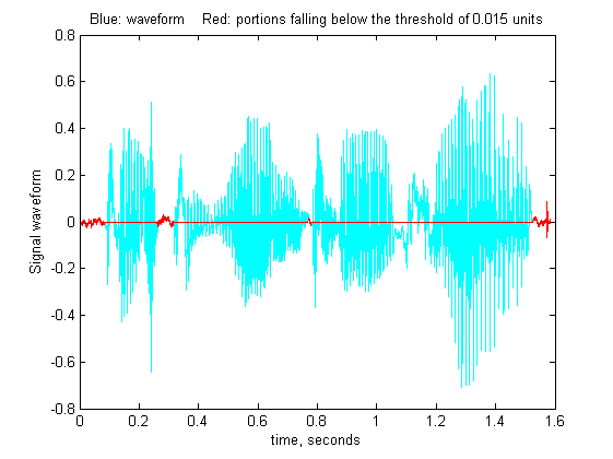
With periodic signal waveforms the situation is a bit more complicated. As an example, consider the audio recording of the spoken phrase "Testing, one, two, three" (click to download in .mat format or in WAV format) that was used previously. The Matlab/Octave script PeriodicSignalSNR.m loads the audio file into a variable "waveform", then computes the average amplitude of the waveform (the "envelope") by smoothing the absolute value of the waveform:
envelope =
fastsmooth(abs(waveform), SmoothWidth, SmoothType);
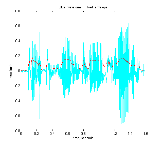
The result is plotted on the left, where the
waveform is in blue and the envelope is in red. The signal is
easy to measure as the maximum or perhaps the average of the
waveform, but the noise is not so evident. The human voice is
not reproducible enough to get a second identical recording to
subtract out the signal as above. Still, there will be often be
gaps in the sound, during which the background noise will be
dominant. In an audio (voice or music) recording, there will
typically be such gaps at the beginning, then the recording
process has already started but the sound has not yet begun, and
possibly at other short periods when there are pauses in the
sound. The idea is that, by monitoring the envelope of the sound
and noting when it falls below some adjustable threshold value,
we can automatically record the noise that occurs in those gaps,
whenever they may occur in a recording. In PeriodicSignalSNR.m,
this operation is done in lines 26-32, and the threshold is set
in line 12. The threshold value has to be optimized for each
recording. When the threshold value is set to 0.015 in the
"Testing, one, two, three" recording, the resulting noise
segments are located and are marked in red in the plot on the
right.
The program determines the average noise level in
this recording simply by computing the standard deviation of
those segments (line 46), then computes and prints out the
peak-to-peak S/N ratio and the RMS (root mean square) S/N ratio.
PeakToPeak_SignalToNoiseRatio =
143.7296
RMS_SignalToNoiseRatio = 12.7966
The frequency distribution of the noise is also
determined (lines 60-61) and shown in the figure on the left,
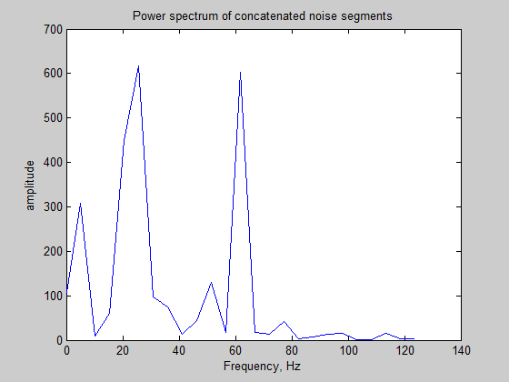
using the PlotFrequencySpectrum function, or you could have used iSignal in the frequency spectrum mode (Shift-S). The spectrum of the noise shows a strong component very near 60 Hz, which is almost certainly due to power line pickup (the recording was made in the USA, where AC power is 60Hz); this suggests that better shielding and grounding of the electronics might help to clean up future recordings. The lack of strong components at 100 Hz and above suggests that the vocal sounds have been effectively suppressed at this threshold setting. The script can be applied to other sound recordings in WAV format simply by changing the file name and time axis in lines 8 and 9.